


Data processing
UKB genotype data
The UKB is a prospective cohort study of approximately 500,000 participants recruited across the United Kingdom from 2006 to 2010 (ref. 18). Phenotype data of anthropometric, biological and lifestyle measures were collected at baseline and in follow-up surveys, with further linkage to health and disease record data. The genetic dataset consists of 488,377 samples genotyped at 805,426 SNPs. To define population ancestries, 4-means clustering analysis was conducted on the first two principal components of the genotype data. Ancestries were then defined according to the country of birth (field ID: 20115) of the majority of individuals in the cluster, resulting in 461,931 European, 11,074 South Asian, 7,935 African, 2,585 West Asian and 2,550 East Asian individuals, and 1,619 individuals in clusters for which there was no majority country of birth.
Subsequent to clustering, standard QC procedures were applied independently to each ancestry cluster. SNPs with a minor allele frequency (MAF) < 0.01, genotype missingness > 0.02 or Hardy–Weinberg equilibrium test P < 10−8 were excluded. Samples exhibiting high levels of missingness or heterozygosity, or inconsistencies in genetic-inferred and self-reported sex, or showing aneuploidy of the sex chromosomes were removed in accordance with recommendations from the UKB data processing team18. For analyses in the general population, a greedy algorithm was used to remove related individuals to maximize sample retention while removing all third-degree relatives (kinship coefficient > 0.044)41. After these QC steps, 411,948 unrelated individuals remained, of whom 387,472 were of European ancestry. The European ancestry cluster included 18,340 individuals with repeated measures that were set aside, as well as 24,476 individuals of multiple non-European ancestries for replication analyses. This resulted in up to 369,132 unrelated individuals of European ancestry for the primary POPout analyses.
For the sibling analyses, sibling pairs were selected by first identifying first-degree relatives, defined as those with kinship coefficient within the range 0.177–0.354 (the expected value for siblings is 0.25) to account for expected variation among siblings42. Only individuals of European ancestry were included in the sibling analyses owing to insufficient statistical power of the multiple ancestries sample2. The proportion of SNPs with zero identity-by-state (IBS0) was used to distinguish sibling pairs from parent–offspring pairs, as parent–offspring pairs have IBS0 ≈ 0 across the autosomes. In the UKB, there is clear separation between pairs of first-degree relatives at IBS0 = 0.00112 (ref. 42); thus, sibling pairs were selected as those exceeding this threshold. This provided a total of 17,289 sibling pairs for analysis.
Quantitative trait QC
Initial trait selection
We considered an initial list of 408 non-procedural continuous traits from the UKB categories of biomarkers, physical measures, the touchscreen questionnaire and cognitive function to provide a broad group of well-studied traits. We removed three traits related to lifetime reproductive success used as outcomes in the selection analyses to avoid circularity, as well as three predicted traits that had directly measured alternatives. To minimize non-genetic causes of trait values, we then removed all individuals with a cancer diagnosis (34,698) and those on insulin treatment (1,311) or who were pregnant at baseline (109). We also removed 64,043 individuals on statins and other cholesterol-lowering drugs from the blood count and blood biochemistry subcategories and 29,395 individuals on heart rate medication from the arterial stiffness and blood pressure subcategories. Next, to ensure that extreme outliers did not affect results, we removed all samples that had trait values six standard deviations or more from the mean. After removal of these samples, we removed traits for which the top two modal values comprised more than half the samples and traits with fewer than 100,000 samples remaining in our primary dataset of unrelated individuals of European ancestry, resulting in a set of 141 quantitative traits. These traits were then residualized and subjected to further QC.
Trait residualization
To minimize the impact of environmental risk factors, we residualized trait values within each ancestry group (European and multiancestry) by applying a linear regression model to each trait, with covariates for age, age2, age3, sex (as reported by the UK National Health Service at birth, unless since revised by the participant), menopause status (among females), type II diabetes status, coronary artery disease status, alcohol intake (field ID: 1558), smoking (categorical, field ID: 20116; continuous, field ID: 1239), batch, centre and the first 40 genetic principal components. At this stage, trait residuals with an absolute skew greater than 2 in the larger European ancestry group were removed to mitigate measurement bias, and the remaining trait values were standardized using a rank inverse normal transform on the residuals. This inverse normal transformation of the traits introduced a conservative bias in the POPout test, although this was expected to be small because of the removal of highly skewed traits and application to trait residuals, and was performed to prevent inflation of the statistic in the linear regression framework of the tests. This provided traits adjusted by key environmental factors and genetic principal components and with relatively low skew, transformed to have standard normal distributions for all subsequent analyses.
GWAS and further QC
For our initial primary analyses, European ancestry UKB samples were split randomly into 50% base and 50% target datasets, for computation of GWAS results and PRS, respectively. Then, for each trait, a GWAS was performed using the standardized trait values in the base data, applying PLINK-1.9 (refs. 43,44), whereas heritability and pairwise genetic correlations were estimated using LD score regression45. To ensure that our PRS analyses were well powered, we removed traits with heritability \(h^2 < 5 \% \) (ref. 19), and to ensure that the traits were essentially polygenic rather than oligogenic, traits were removed for which a single SNP (MAF > 1%) explained more than 2% of trait variance46. We also removed traits on the basis of deviations from trait–PRS linearity in the body of the trait distribution (‘POPout test QC’). After these QC steps, 114 quantitative traits remained across all four categories.
To ensure that the traits were different from each other, for traits with pairwise genetic correlation greater than 0.98, the trait with larger sample size was retained to maximize power for analyses; in addition, for correlated networks of traits, the traits that ensured optimal retention of traits were removed. This led to a further 36 traits being removed. A further four traits were removed on the basis of manual assessment of retained traits, as genetic correlation can be underestimated between traits with large differences in sample size. Together, these steps resulted in a set of 74 traits for use in the primary analyses. This broad set of traits ensured comprehensive coverage over a diverse set of phenotypes and provided adequate numbers of overlapping traits for the replication analyses.
Using scripts provided (‘Code availability’) researchers can perform this QC pipeline or change the QC thresholds to produce bespoke analyses, with information output on the traits that are removed and retained at each stage, and generate a full set of results.
PRS calculation
The 74 traits remaining after QC comprised 35 traits in the biomarkers category, 24 traits in the physical measures category, and 15 that were in either the touchscreen questionnaire or the cognitive function category. In the primary unrelated European dataset, these traits had between 50,109 and 167,857 (mean 123,482) samples in each of the base and target datasets. For each (residualized) trait, PRSice-2 (ref. 47) was used to calculate PRSs for all individuals of the target data (second half of data), using base data GWAS (see above) and the FastScore option, which selects the optimal PRS from one of ten P value thresholds. Each PRS and corresponding trait was then used in the POPout analyses.
The POPout test was performed in the target sample, that is, the sample in which the PRSs were trained, to optimize sample size for testing in the tails. Although each PRS was fitted (by means of P value threshold optimization) to the same data used for POPout testing, the use of only ten P value thresholds was expected to minimize this overfitting to the target sample; this is a conservative bias in any case, because the PRSs were fitted assuming a linear relationship between the PRS and trait. None of the replication analyses (below) was subjected to any overfitting as they all corresponded to out-of-sample data.
Replication datasets
European ancestry repeated measures
After initial QC of the UKB sample (above), there were up to 18,340 European ancestry individuals with measurements repeated at a follow-up data collection an average of approximately 5 years after baseline (timing differed for different individuals) for 63 of the 74 traits from the primary analysis. For these individuals, both measurements were normalized alongside the other European ancestry UKB samples, as described above, but held out of the base dataset. Then, the residualized trait values from their two visits were averaged (mean) to provide a target subset of individuals for whom random measurement error or transient effects (for example, infections) were less likely to produce trait values in the tail. For the 63 traits, there were between 2,461 and 15,475 unrelated individuals with repeated measures available for replication.
Multiancestry sample
After initial QC, there were up to 24,476 individuals of multiple ancestries (in order of sample size: South Asian, African, West Asian, East Asian and other smaller sized ancestries; see ‘UKB data’ section for classification of ancestries) available for replication; we refer to this sample as the multiancestry replication sample. The trait values of these individuals were normalized alongside those of the European UKB individuals, and PRSs were calculated for the 74 traits of our primary analyses using PRSice-2 (ref. 47). PRSs were calculated in this sample using the P value threshold (and thus the same SNPs) optimized for the relevant trait in the primary analyses, as well as the (same) effect size weights of the base GWAS. There were between 569 and 22,513 unrelated individuals for this multiancestry replication.
All of Us cohort
The All of Us Research Program is a diverse ancestry biobank from the United States, using electronic health record data in a cohort of individuals with a wider age range than the UKB (mean (s.d.) age of 55.8 (17.1) versus 56.5 (8.1) years). Traits matching those studied in our primary UKB analysis were identified through an initial database search and then interrogated manually to determine whether trait descriptions were sufficiently similar. We identified 31 traits as overlapping with the 74 traits of the primary UKB analysis, available for replication here. All of Us provides ancestry categories that correspond to the labels used in gnomAD48 and are based on principal component analysis projection of samples into the principal component analysis space of the training data comprising the Human Genome Diversity Project49 and 1000 Genomes project50. A total of 133,581 individuals of European ancestry (genetically inferred by All of Us) were extracted for analysis. Trait QC in All of Us was conducted to match that performed in the UKB as closely as possible, given available trait information. First, individuals on statins were removed from the blood count and blood biochemistry subcategories; then, the median measurement value for every trait (electronic health record data includes multiple measures) was selected, and the age corresponding to that measurement was extracted. For each trait, outliers more than six standard deviations from the mean were removed, and a linear regression model was applied with covariates for age, age2, age3, sex (reported at birth) and the first 40 genetic principal components. A rank inverse normal transformation was applied to the regression residuals to provide standardized trait values, as for the UKB.
Genetic QC in All of Us was conducted using standard filters, as used in the UKB. SNPs with MAF < 0.01, genotype missingness > 0.02, or Hardy–Weinberg equilibrium test P < 10−8 were excluded. The same greedy algorithm used to maximize sample retention of unrelated individuals in the UKB was applied here. Using the higher-powered publicly available European ancestry GWAS summary statistics generated from the entire UKB40 to provide SNP weights, we calculated trait PRSs47 using the same P value threshold relevant to each trait and trained in the UKB European ancestry analysis.
POPout analyses
The POPout test
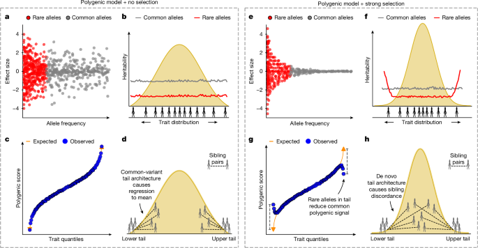
The POPout test was designed to identify departures from common-variant architecture in the tails of quantitative traits from population genotype data. In our application, we sought to identify departures due to genetic factors; thus, we first performed regression of traits on environmental risk factors and used the residuals as input to the test. The POPout test first applies a regression of PRS-on-trait values, in which both the PRS and trait are standardized to have a standard deviation of 1. The assumption of the test is that under uniform and predominant common-variant architecture, comprising many common variants of small effect, there is a linear relationship in prediction of PRS from trait values, whereas under reduced common-variant architecture in the tails, the fitted regression values systematically overestimate the absolute PRS values in the lower and upper quantiles (that is, the observed PRS for extreme trait values is closer to the population mean PRS than predicted by linear regression). The residuals from the regression are evaluated in trait quantiles (centiles here), and two-tailed t-tests are applied to test whether the residuals are significantly different from zero. Here we applied the test to individuals in the lower and upper 1% of the trait distribution to test for departures from common-variant architecture in the tails. The POPout effect size in each tail was defined such that a positive effect was indicative of regression to the mean in both the lower and upper tails, as follows:
$$\textPOPout effect\,=\,\frac1n\mathop\sum \limits_i^nf(\,y_i)-\textPRS_i.(\textsign(\,f(\,y_i))),\,i\in 1,\ldots ,n:y_i > K,$$
where \(K=\varPhi ^-1(0.99)\) (testing the top 1% tail), \(\varPhi ^-1\) is the inverse normal cumulative density function, \(f(\,y_i)\) is the predicted PRS from the regression given trait value \(y_i\) and n is the number of observations in the quantile.
POPout test QC
A further trait QC was applied to ensure the robustness of the POPout to its assumptions by ensuring that the POPout test did not produce significant results in the middle of the trait distribution. Specifically, for each trait, two-sided t-tests for zero mean were applied to the residuals assigned in each of the middle 80 centiles of the trait distribution. Traits were deemed to fail QC if the smallest P value was significant at a Bonferroni-corrected level of 0.05 (P ≤ 0.05/80). Three traits were removed on the basis of this criterion in our large UKB primary analysis, six of the repeated measures traits, ten traits in the multiancestry replication and three traits in All of Us.
Replication of POPout effects
We replicated our primary POPout analyses in three different independent cohorts: (1) UKB European ancestry individuals with repeat measures (baseline and follow-up at approximately 5 years), (2) non-European multiancestry UKB individuals combined into a single group, and (3) the European ancestry samples in the US-based All of Us biobank. Replication POPout analyses were then performed in cohorts (1) and (2) using the PRS models trained in the primary analysis (that is, the same variants and effect size weights for the PRS), and likewise for cohort (3) except that the effect size weights of the variants were derived from the total UKB sample of individuals with European ancestry, as the All of Us sample is entirely independent and thus cannot be subject to overfitting.
In our primary analysis, we set a minimum total sample size threshold of 100,000 (at least 50,000 target samples). To set an appropriate minimum sample size for replication, we explored the power of POPout at different sample sizes, applying POPout to subsets ranging from 1,000 to 50,000 target samples, with subset sizes incremented by 5,000 (Extended Data Fig. 3). Analyses were repeated 100 times for each sample size. Results were compared with the primary analysis with respect to (1) the number of false discovery rate 5% significant tails replicated at P < 0.05 and (2) the average (Pearson) correlation across POPout effects between the primary and subset analyses. As shown in Extended Data Fig. 3, at subset sizes of 5,000, the mean correlation across bootstraps was 0.72, whereas at a sample size of 1,000 the mean correlation was 0.41. A threshold of 5,000 was therefore used as a minimum for each cohort in the replication analyses.
After performing the POPout test QC and applying a sample size threshold of >5,000 individuals, we had 50 traits (of 63 overlapping traits) for the repeated measures replication across an average of approximately 12,000 individuals, 55 traits (of 74 traits) for the multiancestry replication across an average of approximately 17,500 individuals, and 27 (of 31 overlapping traits) for the All of Us replication across an average of approximately 53,000 individuals.
Evaluating impact of POPout effects on PRS accuracy
To evaluate how observed POPout effects affected the performance of PRS prediction, we emulated a scenario in which the quantitative trait underlies a binary outcome (for example, body mass index underlying clinical obesity). We considered individuals above a specified trait threshold value to be cases and individuals below the threshold to be controls. We investigated thresholds at the 75% and 99% points of the trait distribution. For each, we used the PRS to predict case or control status and then generated a quantile plot in which the odds ratio of the given quantile was estimated in relation to the central quantile by means of logistic regression (Fig. 2c). In addition, for each trait with PRS r2, we simulated a quantitative phenotype with trait values given by \(T=r\rmP\rmR\rmS+E\), where PRS has a standard normal distribution and \(E\) represents all other contributions to trait variance and is drawn from a normal distribution with mean 0 and variance \((1-r^2)\). This produced a simulated trait with \(\mathcalN(0,1)\) distribution and PRS r2. Using the same number of target samples as in the real data analysis for each trait, this simulation allowed us to estimate the expected predictive performance of the PRS on the basis of the corresponding r2, assuming uniform polygenicity throughout the trait distribution. The results of this analysis for all our index traits are shown in Extended Data Fig. 2.
Sibling-based analyses
Sibling-based investigation of departures from common-variant architecture
We previously developed sibling-based tests of departures from polygenic expectations in trait tails caused by de novo high-impact alleles or rare alleles of large effect segregating in families (Mendelian effects)2. Here we summarize the theoretical framework underlying those tests and describe the single omnibus test used here that combines the two tests to identify general departures from common-variant architecture due to either cause.
The conditional distribution of an individual’s trait value given their sibling’s trait value, assuming the infinitesimal model for genetic effects (common-variant architecture) and normally distributed environmental factors, can be derived analytically2 as
$$p(s_2|s_1) \sim \mathcalN\,\left(\frac12s_1h^2,1-\frach^44\right),$$
where \(s_1\) and \(s_2\) denote the index and conditional-sibling trait values, respectively, and \(h^2\) is the trait heritability. Rare large-effect alleles can produce deviations from this distribution, particularly when concentrated in specific parts of the distribution, as may occur in the trait tails if these effects are very large and abundant. Specifically, rare large-effect alleles segregating in families (Mendelian effects) will result in excess trait similarity (or concordance) between siblings on average compared with a common-variant only architecture. Conversely, a high-impact de novo mutation in one sibling will result in excess dissimilarity (discordance) between siblings.
Our sibling-based test for enrichment of Mendelian effects2 evaluates the proportion of sibling pairs in which both siblings reside in a defined quantile of the trait distribution; this can be formulated as a score test with the following z-statistic:
$$z=\fracr-n\pi _\sqrtn\pi _(1-\pi _),$$
where \(n\) is the number of index siblings in quantile \(q\) under test, \(r\) is the number of sibling pairs in which both siblings have trait values in \(q\). \(\pi _\) is the expected proportion of sibling pairs in the quantile under common-variant architecture, given by:
$$\pi _=\frac1n\sum _i\in A_q\left(1-\varPhi \left(\frac\varPhi ^-1(q)-\fracs_1^(i)h^22\sqrt1-\frach^44\right)\right),$$
where n is the number of sibling pairs, \(A_q\) is the set of index siblings in trait quantile q, \(\varPhi \) is the normal cumulative density function and \(\varPhi ^-1\) is its inverse.
Our sibling-based test for enrichment of de novo effects constructs a z-statistic for the distance between index siblings in the tail of the trait distribution and their conditional siblings, as follows:
$$z=\frac\sum _i\in A_qs_2^(i)-\frac12s_1^(i)h^2\sqrtn\left(1-\frach^44\right).$$
For index siblings in the lower and upper tails, the alternative hypotheses of \(H_1:z > 0\) and \(H_1:z < 0\) are tested as one-tailed t-tests, respectively. For further details, see Souaiaia et al.2.
The trait heritability, \(h^2\), a required parameter in the Mendelian and de novo tests, is estimated from the sibling pairs by calculating the maximum likelihood of \(h^2\) under the null hypothesis of the infinitesimal model:
$$\log \mathcalL\propto -n\log \left(1-\frach^44\right)-\frac11-\frach^44\mathop\sum \limits_i=1^n\left(s_2^(i)-\fracs_1^(i)h^22\right)^2.$$
The sibling STANDout test
To test for general departures from common-variant architecture in the tails of quantitative traits, caused by high-effect alleles that are either de novo or segregating in families (that is, rare alleles), we combine the results of the two tests using Fisher’s method to give a \(\chi ^2\) statistic with four degrees of freedom:
$$\chi _4^2=-2(\rml\rmo\rmg(P_\rmM\rme\rmn\rmd\rme\rml\rmi\rma\rmn)+\rml\rmo\rmg(P_\rmdenovo)).$$
Analysis of rare variants
Calculating associations between POPout effects and rare exome hits
Backman et al.26 provided association results from the UKB exome sequencing study across 3,994 traits. These results included 65 of the 74 traits analysed in our target set. For each of these 65 traits, in each tail, we counted the number of genes with at least one significant association. Following Backman et al.26, we defined gene significance as either a single-variant deleterious, missense or predicted loss-of-function association, or a gene-burden association, at P \(\le \,2.18\times 10^-11\). Across the 130 trait tails, we calculated the Pearson correlation between the number of genes with significant exome associations and the POPout effect size.
WGS data to identify rare variants
The UKB recently released WGS data for approximately 500,000 participants27. This dataset has an average coverage depth of 23.5×, enabling reliable detection of rare genetic variants (MAF < 1%) typically absent from PRS analyses. We analysed the European-ancestry samples that had previously undergone QC using the same standardized 74 traits. GWAS (with standard QC filters, variant missingness < 0.02), followed by clumping and thresholding (\(r^2=0.1\), window: 250 kb) were applied using PLINK-1.9 to identify independent rare associations43,44 with 0.01% < MAF<1% in the full dataset. In addition to the covariates used in the common-variant GWAS, the top 40 rare-variant principal components were included as covariates in the GWAS, after which independent variants meeting the criteria for genome-wide significance (\(P < 2.18\times 10^-11\)), as described by Backman et al.26, were retained and separated into two groups on the basis of MAF. Variants in each group were summed across sample genotypes to build moderately rare (0.1% < MAF < 1%) and very rare (0.01% < MAF < 0.1%) PRS models for each trait.
WES data to identify rare burden variants
The UKB has released WES data for over 450,000 of 500,000 participants26, enabling gene-level burden variants to be tested for association with quantitative traits. For the 40 traits with at least one genome-wide significant rare-variant and significant positive POPout, we used interim-release PLINK-format WES data that had undergone QC to further identify burden variants. First, we applied REGENIE v.4.1 (ref. 51) to fit chromosome-level whole-exome REGENIE null models (REGENIE step 1) using all available samples (passing our original QC) and a pruned set of high-quality variants (MAF > 1%, LD pruning window: 50 kb, \(r^2 < 0.2\)) to generate leave-one-chromosome-out predictions that controlled for population structure and relatedness.
Next, we performed gene-based burden testing (REGENIE step 2) in the base sample subset (in which GWAS were performed in the primary analyses) using leave-one-chromosome-out predictors from step 1 and the standard four functional masks defined in the UKB exome files, capturing rare (MAF < 1%) and singleton loss-of-function and damaging missense variants. Burden effect sizes (\(\beta \)) and corresponding P values were obtained for each gene–mask pair. To avoid double-counting of rare variants within traits, we excluded gene–mask pairs containing variants overlapping with our single-variant rare PRS analysis, which will have reduced the specific power of our burden-based analyses (but not the power of the overall rare-variant analyses). Next, we selected the most significant mask per gene, consistent with standard burden-based frameworks26,52, and retained those with P values exceeding genome-wide significance (\(P < 2.18\times 10^-11\))26. Per-sample burden genotype matrices for individuals in the target sample (the second half of the UKB sample used for POPout analyses) were then multiplied by the corresponding burden \(\beta \) coefficients and summed across chromosomes to compute burden-variant PRS in the target sample for each trait.
Construction and analysis of common + rare PRS
For each trait, the union of target samples from our original common-variant PRS and samples available in the WGS and WES datasets (more than 99% of sample shared) were used to calculate a combined common + rare PRS that was summed across common risk scores (\(MAF > 1 \% \)), moderately rare single-variant risk scores (\(0.1 \% < MAF < 1 \% \)), very rare single-variant risk scores (\(0.01 \% < MAF < 0.1 \% \)) and burden-variant risk scores. For the 40 traits (of 74 traits in total) with significant rare variants identified and positive POPout effects, common-variant PRSs were used to recalculate POPout effects in the overlapping samples (with genotype, WES and WGS data), and common + rare-variant PRSs were used to calculate new POPout effects that incorporated rare variants. To compare these POPout values, we quantified the ‘POPout reduction’ as follows:
$$\textPOPout\,\textreduction\,=\,\frac\rmPOPout_\rmcommon-\rmPOPou\rmt_\rmcommon+\rmrare\rmPOPou\rmt_\rmcommon$$
and evaluated whether the reduction was statistically significant using a one-sided paired t-test on the within-individual differences between POPout effects.
In the odds ratio analyses, odds ratios were calculated for PRS prediction of a hypothetical disease defined as corresponding to the lower or upper 1% tail, for each trait tail before and after inclusion of rare variants (that is, corresponding to odds ratios calculated using only the common PRS versus odds ratios calculated using the common + rare PRS).
Selection analyses
Forward-in-time population genetic simulations
Using SLiM v.4.0 (ref. 17), we simulated a quantitative polygenic trait under a standard Wright–Fisher model of stabilizing selection. First, a population of N = 10,000 diploid individuals of genome size 100 kb was simulated to equilibrium (N generations; as well as sensitivity analyses of 5N and 10N generations) with a constant mutation rate of \(2.36\times 10^-8\) per base pair and recombination rate of \(10^-8\) per base pair under neutrality. Mutations were assigned effect sizes simulated from a gamma distribution with shape parameter 0.186 and mean of 0.01026 and subsequently multiplied by −1 with probability 0.5 to give a symmetrical effect size distribution. This distribution has been used previously to simulate genetic effects in humans and reflects a prior belief in a small number of large effects and many small effects53. In sensitivity analyses, gamma distributions with means of 0.005, 0.01 and 0.02 (shape 0.186), as well the standard Gaussian distribution, were used instead for the effect sizes. Individual trait values were determined by the sum of all genetic effects, corresponding to full heritability (\(h^2=1\)).
After neutral genetic diversity had been achieved (10N generations), stabilizing selection on the trait was introduced for N (5N, 10N in sensitivity analyses) generations through a Gaussian fitness function
$$f_t(x)=1+\frack\sqrt2\pi \sigma ^2\exp \left\-\frac(x-\mu )^22\sigma ^2\right\,$$
where k is a multiplier for strength of selection, x is the phenotype of an individual at generation t, and \(\mu \) and \(\sigma \) are the trait mean and standard deviation at the start of selection (that is, \(t=10N\)).
We ran this simulation for 100 independent replicates and reported data in each simulation by logging, at each generation, the phenotypic mean and standard deviation of the population, as well as statistics related to the mutations present in the populations, including allele frequencies and effect sizes, and the mutational profile of each individual. To analyse the enrichment of rare-variant architecture at different quantiles, the population was stratified across 100 centiles (each including 100 individuals), and the number of rare and common alleles carried by individuals in each centile was calculated under neutrality versus under selection. For comparison purposes, ‘weak selection’ corresponded to simulations performed using a multiplier of \(k=1\) in the fitness function equation above, whereas ‘strong selection’ corresponded to simulations with \(k=100\). ‘Large effects’ were considered to be those in the top 10% of effect sizes genome-wide. The mean of the log-transformed odds ratio across all 100 independent simulation replicates was used as a measure of enrichment, and a t-test was performed to test for significant differences from zero. To analyse the impact of low-frequency variants on prediction and mimic the calculation of common-variant PRS in real data, a PRS was calculated using only variants with MAF > 1% and compared with the true trait value across the individuals in each centile. The mean difference (POPout effect) and 95% confidence intervals in each centile were calculated across the 100 independent simulation replicates. These simulations reflect a subset of those performed in a recent simulation study that we conducted54.
Inferring selection on the basis of relative lifetime reproductive success
The number of offspring is recorded in the UKB for both females and males. Following the approach of Beauchamp55, samples were stratified into four birth cohorts (1934–1942, 1943–1948, 1949–1955, 1956–1965). Individual relative lifetime reproductive success, \(Y_\rmrLRS\), was then calculated by dividing the number of offspring of each individual by the cohort mean. Following Sanjak et al.16, we inferred the presence and direction of selective pressure acting on traits by fitting the following regression model:
$$Y_\rmrLRS=\beta _+\beta z+\gamma z^2,$$
where z denotes the residualized and normalized trait values, and \(\beta \) and \(\gamma \) are linear and quadratic regression parameters.
We used the BIC to select the best-fitting model for each trait, from which the selective pressure acting on each trait was inferred. If the selected model did not include a linear or quadratic parameter, then no selection was inferred. If the selected model included only the linear term, then negative selection was inferred if \(\beta < 0\), whereas positive selection was inferred if \(\beta > 0\). If the selected model did not include a linear term but included the quadratic term, then stabilizing selection was inferred if \(\gamma < 0\), suggesting that the mean trait value in the population was optimal; if instead \(\gamma > 0\), it was considered that both tails of the distribution were subject to positive selection (this is known as ‘disruptive selection’ and is expected to be rare in practice). When the BIC-selected model included both linear and quadratic terms, the \(\beta \) parameter was used to indicate the general direction of selection as positive or negative, and the quadratic term was considered to suggest that an optimal mean was being reached.
Association between POPout effects and lifetime reproductive success
To test the association between POPout effects and the selection acting on corresponding traits as inferred by the lifetime reproductive success model, we stratified traits into four categories of selection. The first two of the four categories reflected non-directional selection: (1) no selection (\(\beta =0,\gamma =0\)), in which POPout effects were not expected in either tail; and (2) non-directional stabilizing selection (\(\beta =0,\gamma < 0\)), in which we expected POPout effects in both tails of equal magnitude. The third and fourth categories reflected directional selection: (3) positive selection (\(\beta > 0\)), which could be linear (\(\gamma =0\)), disruptive (\(\gamma > 0\)) or stabilizing (\(\gamma < 0\)), in which we expected greater POPout effects in the lower tail versus the upper tail; and (4) negative selection (\(\beta < 0\); linear, disruptive or stabilizing as for positive), in which we expected greater POPout effects in the upper tail versus the lower tail. For each category, a t-test was used to test for the difference in mean POPout effects (excluding non-significant POPout effects) between the lower and upper tails across the traits.
Sensitivity of lifetime reproductive success analyses to BIC model choice
For each pair of best and second-best models, as ranked by BIC, we performed the following comparison. When the second-best model was a nested subset of the best model, we calculated the likelihood ratio test to determine whether it was significantly better-fitting (P < 0.05). When the second-best model had more parameters, we determined that a difference in BIC of less than 2 was weak evidence of model superiority56. These two criteria identified ten and seven traits, respectively, for which there was justification to test the second-best model. These traits are shown in the Supplementary Information. In sensitivity analyses, we also replaced the best model with the second-best model for these 17 traits and then re-estimated the relationship between LRS and POPout effects observed in Fig. 5d (Supplementary Information).
Calculating association between POPout effects and fitness measures
Five broad measures of fitness were considered: (1) male and (2) female fecundity (field IDs: 2405 and 2734), (3) self-reported non-cancer illnesses (field ID: 2002), (4) total miscarriages and stillbirths (field IDs: 39290 and 3839), and (5) paternal age (calculated as the difference between father’s age (field ID: 2946) and participant age (field ID: 21022)). The association between each of these measures and the POPout effects was calculated across the lower and upper (1%) tails, as in the following example. To test for the association between paternal age and POPout effects, the mean paternal age of the individuals residing in the upper tail and lower tail was calculated for each of the 74 traits, resulting in a set of 148 mean paternal age values. These 148 values were then tested for their associations with the corresponding 148 POPout effect sizes (two POPout effects, one for each of the lower and upper tails, across the 74 traits) using Spearman’s rank correlation. All analyses and QC described here can be repeated, modified or expanded using our publicly available scripts57.
Reporting summary
Further information on research design is available in the Nature Portfolio Reporting Summary linked to this article.

