


Ethical approval and sample collection
All necessary ethical approvals to conduct this work and to ensure that the derived organoids could be used for academic and commercial purposes were obtained from each participating clinical site for the collection of patient samples as well as for the Wellcome Sanger Institute for organoid derivation (IRAS ID:203519; REC 16/LO/1110). Further details are provided in Supplementary Information.
Availability of Organoid Biobank
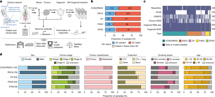
Organoids have ethical approval for use in academic and commercial purposes. Models are being distributed by American Type Tissue Culture (ATCC) as part of the HCMI collection (https://www.atcc.org/hcmi) and EMD Millipore. Repository details and model availability are provided in Supplementary Table 2.
Organoid derivation
Detailed protocols for organoid derivation, cryopreservation and routine culturing are published on protocols.io and include embedded demonstration videos and workflow diagrams62,63,64. Tumour samples were washed 3 times with PBS, minced, and either cryopreserved after centrifugation (800g, 2 min)63 or enzymatically digested for 1–2 h at 37 °C. The suspension was filtered (100 μm), centrifuged and washed to remove debris and digestion buffer62. Isolated cells were embedded in approximately 15 μl droplets of extracellular matrix (80:20 basement membrane extract (BME):medium; 6.4–9.6 mg ml−1 protein; Cultrex BME Type 2 Select 3532-001-02) and plated in pre-warmed 6-well plates following established protocols64. After polymerization (15–20 min, 37 °C), 2 ml of organoid medium prepared using established recipes39,65,66,67 was added, supplemented with antibiotics and 1 μl ml−1 ROCK inhibitor (Y-27632, Staratech Scientific S1049-SEL-5mg).
After expansion to ≥25 million cells, 25 cryovials were banked and pellets collected for sequencing. Post-thaw viability was confirmed by re-culturing for four passages with freeze–thaw quality control assessment.
Organoid culture
Organoids were maintained either in 80% BME-2 droplets or in 5% BME-2 suspension culture38. In the 80% BME-2 culture, organoids were cultured as described above. For the 5% suspension method, cancer organoids were suspended in a medium/extracellular matrix (ECM) dilution. For example, combining 10 ml of medium with 500 μl of BME-2 achieved the desired concentration, and organoids were then cultured in ultra-low-adherent flasks or plates.
For passaging, the medium, cells and ECM were collected and centrifuged at 800g for 2 min. After discarding the supernatant, organoids were dissociated using TrypLE (Gibco 12604013), an enzymatic reagent. The suspension was incubated for 10–60 min, allowing dissociation into small clumps. The cells were then pelleted and replated as described64.
Model identifiers
All models presented in this study have a sanger_ID starting with ‘WTSI’, corresponding to the Wellcome Trust Sanger Institute. Additionally, if a model is shared with the HCMI, it also has an HCMI ID starting with ‘HCM’. When both IDs are available, the HCMI nomenclature is used as the sample_ID. The equivalences are shown in Supplementary Table 2.
Whole-genome sequencing and analysis
Sequencing and alignment
DNA extracted from snap-frozen tumour tissues, snap-frozen organoid cell pellets, blood or formalin-fixed paraffin-embedded normal tissues samples were prepared for WGS. Whole genome paired-end sequencing reads (150 bp) were generated using the Illumina HiSeq X Ten platform with an average coverage of 38×, comparable to coverage used for PCAWG. Reads were aligned using the BWA-MEM (v0.7.17) tool68. PCR duplicates, unmapped and non-uniquely mapped reads were filtered out before downstream analysis.
SNV and indel calling
Somatic SNVs and short indels were identified using cgpCaVEMan69 and cgpPindel70, respectively. Germline variants and artefacts were filtered using matched normal samples and a panel of normals, with further post-processing using cgpCaVEManPostProcessing (https://github.com/cancerit). Variant allele frequencies (VAFs) were estimated using vafCorrect (v2.4.0)71, and variants with VAF > 0.05 were retained. Further details in Supplementary Information.
Structural variant and copy number calling
Copy number and allele-specific information were derived using AMBER (v3.5)72 and COBALT (v1.11)72. Somatic and germline SNVs and indels were identified using SAGE (v2.8) and SnpEff (v5.0)73. Somatic SVs were called using GRIDSS2 (v2.12.0)74, annotated with RepeatMasker (v4.1.2)75 and kraken2 (v2.1.2)76, and filtered with GRIPSS (v1.9)77. Subsequently, this information was integrated to calculate the microsatellite status, tumour purity, ploidy, WGD and SCNAs using PURPLE (v2.54)72. SCNAs were converted into discrete copy number states. SAGE, GRIPSS, AMBER, COBALT and PURPLE were developed by the Hartwig Medical Foundation (HMF) (https://github.com/hartwigmedical/hmftools). Further details in Supplementary Information.
Cancer driver event annotation
We compiled a list of 783 cancer driver genes, derived as the union of two complementary gene sets from the IntOGen78 and COSMIC79 databases, as previously reported9. Each gene was annotated by its mechanism of action as either activating (Act, for oncogenes), loss-of-function (LoF, for tumour suppressor genes), ambiguous (with evidence of both mechanisms), or fusion. The complete list of cancer driver genes is in https://cellmodelpassports.sanger.ac.uk/downloads.
We collated individual putative cancer driver mutations (for example, frameshift, nonsense, stop-lost, exonic splicing silencer, missense or in-frame mutations) among SNVs and indels within these cancer driver genes from four data sources: IntOGen (including Cancer Genome Interpreter and BoostDM)78, MSKCC80, and cancer predisposition variants, that were identified by overlap with a reference set of pathogenic germline variants with matching effect81.
Loss of heterozygosity
We considered a tumour suppressor gene or an ambiguous gene to have loss of heterozygosity if the DNA copy number (CN) of the minor allele was <0.5 and the difference between the round ploidy and the round total CN was >0 (there was no amplification in the non-mutated allele) or if the VAF of a loss-of-function mutation was >0.85.
Biallelic alterations
Biallelic alterations included all cases with loss of heterozygosity, as well as homozygous deletions, SV disruptions or instances where each allele was affected by a different loss-of-function mutation.
Multiplicity, CCF and clonal mutations
SNVs were intersected with segment SCNAs using the GRanges and findOverlaps functions from the GenomicRanges R package (v1.56.1) to obtain information on the major allele, minor allele, and total tumour CN for each SNV, along with the VAF and tumour purity. The multiplicity (the number of chromosomal copies harbouring a given mutation) and CCF (the proportion of cancer cells carrying a specific mutation within a tumour sample) were then calculated according to the formulas in Steele et al.82 and Dentro et al.83. Clonal mutations, defined as genetic alterations present in all cancer cells within a tumour, were identified as those with a CCF > 0.75.
CN correlation between paired organoids and tumours
SCNA segment data was divided into 100 kb bins across the genome, and the CN for each segment was calculated as the mean CN of all positions within the 100,000 bp window. Positions listed in the ENCODE blacklist84 (https://github.com/Boyle-Lab/Blacklist) were excluded from this analysis. Pearson correlations were then computed using the mean CN for each segment between paired organoid and tumour samples.
Focal amplifications
Focal amplifications were defined as the presence of at least two genomic segments, each exceeding 100 kb in size, with a log2(CN/ploidy) value > 6.
Signature analysis
Mutational signatures were extracted using SigProfilerExtractor (v1.2.2)85 for the tumour and organoid samples from each tumour type separately. COAD/READ-MSI samples were analysed separately from COAD/READ-MSS samples. STAD samples were not analysed due to insufficient sample size. The resulting matrix file was used as an input for SigprofilerAssignment (v0.2.5)30 to assign known COSMIC v3.4 signatures within single base substitution (SBS). De novo signatures were further refitted using the COMICv3.4 and an additional set of novel CRC and MSI specific signatures identified and validated in Mutographs project86.
For data visualization, COSMIC mutational signatures representing less than 10% of mutations within each sample were categorized as ‘Others’ and excluded from calculations of both the proportion of models with that mutational signature and the proportion of mutations representing each signature by cancer type. SBS5 and SBS40a were collapsed into a single category, based on the hypothesis that these signatures arise from a combination of correlated mutational processes87,88.
Homologous recombination deficiency
Homologous recombination deficiency was assessed using CHORD (v2.0.3)34.
Complex genomic rearrangements
Chromothripsis and other complex genomic rearrangements were detected using ShatterSeek (v1.1)26, as previously described89.
RNA-seq and analysis
Paired-end transcriptome reads (75 bp) were quality filtered and mapped to GRCh38 (ensemble build 98) using STAR (v2.5.0c)90 with a standard set of parameters (https://github.com/cancerit/cgpRna). Resulting bam files were processed to get the per gene read count and transcripts per million (TPM) data using RSEM (v1.3.3)91. TPM values were used for the downstream analysis.
CMS/CRIS subtypes
Consensus molecular subtypes (CMS) and colorectal cancer intrinsic subtypes (CRIS) subtypes were inferred for COAD/READ organoids with CMSCaller36,92 using RSEM expected count data.
CRISPR–Cas9 screening
Detailed protocols including process diagrams and example data for generating Cas9-expressing organoid cultures and CRISPR–Cas9 library transduction in organoid are published on protocols.io93,94. Stable Cas9-expressing organoids were generated using lentiCas9-Blast (Addgene 52962) with polybrene (8 μg ml−1). Following overnight incubation, medium was replaced with complete medium containing Y-27632 (2.5 μM), and blasticidin (Invivogen, ant-bl-1, 10 mg ml−1) selection was applied 120 h after transduction. Cas9 activity was measured using a fluorescent reporter assay (Addgene 67982 and 67981)95. Only organoid lines with activity of 75% or more were selected for single guide RNA (sgRNA) library transduction.
Two genome-wide CRISPR–Cas9 sgRNA libraries were used. The Human CRISPR Library Yusa v.1.1 (ref. 3), containing 100,086 sgRNAs that target 18,009 genes (with 5–10 sgRNAs per gene) and 1,004 non-targeting sgRNAs; and the Minimal Genome-Wide Human CRISPR–Cas9 Library (MinLibCas9, Addgene 164896)41, which includes a selected sgRNA primarily drawn from Yusa v1.1 comprising 37,522 sgRNAs that target 18,761 genes (with 2 optimal sgRNAs per gene) and 200 non-targeting sgRNAs (Extended Data Fig. 8a). Lentiviral volume required for multiplicity of infection of 0.3 was determined by titration, and transduction efficiency assessed by BFP flow cytometry.
A total of 12.5 × 10⁸ (Yusa v1.1) or 3.3 × 10⁷ (MinLibCas9) cells were transduced in triplicate using the same batch of Cas9-transduced organoids. No significant batch effects were observed across independent batches of Cas9-expressing organoid lines (Extended Data Fig. 8b). Cells were infected with the lentiviral-packaged whole-genome sgRNA library (for 100× coverage), in medium containing polybrene (8 μg ml−1), and Y-27632 (2.5 μM). Following overnight incubation, cells were plated in fresh medium in a 5% suspension. Transduction efficiency (target of 30%) was confirmed on day 6. Screens were maintained under puromycin selection (Invivogen, ant-pr-1, 10 mg ml−1) for a further 16 days (21 days in screen in total). A final selection efficiency of at least 60% was required for the screen to pass. At the end of the screen approximately 2.5 × 10⁷ cells were collected, pelleted, and stored at −80 °C for downstream processing.
CRISPR screen data processing
CRISPR screens performed using the Yusa v1.1 (ref. 3) and MinLibCas9 (ref. 41) libraries were harmonized by restricting analyses to shared sgRNAs, enabling integrated downstream processing. Quality control procedures, adapted from established cell line screening pipelines3, were applied to assess replicate concordance, sgRNA representation and classifier performance in distinguishing essential from non-essential genes. Low-quality replicates and organoids failing predefined quality control criteria were excluded prior to further analysis. Read counts were normalized and corrected for copy-number effects using CRISPRcleanR (v3.0.1)96, followed by batch correction across libraries97. Gene-level fitness effects were estimated using BAGEL (v2)45 with curated reference gene sets, and LFC values were scaled relative to essential and non-essential controls to facilitate cross-organoid comparability. Full details of sgRNA selection, quality control thresholds, normalization, batch correction, statistical procedures and final selection of models are provided in the Supplementary Information.
CRISPR screen processed data analysis
Analysis of organoid core fitness genes
We applied ADaM implemented in the CoRe R package (v1.0.0) (https://github.com/DepMap-Analytics/CoRe)98 using the same curated reference essential gene set as previously mentioned3 to calculate false-positive rates. This analysis identified 751 core essential genes (Supplementary table 4). Although we used all organoids together as input, only three cancer types were included (PAAD and STAD organoids were excluded), so the resulting core fitness genes do not represent a pan-cancer set.
We compared core fitness genes in organoids with those identified in cell lines9 and observed an overlap of 654 genes, with 97 genes identified as organoid-specific (Extended Data Fig. 9). We performed a Fisher’s exact test on these organoid-specific core fitness genes to perform pathway enrichment analysis, using Gene Ontology Biological Processes, KEGG pathways99 and Hallmarks100 obtained from the msigdbr R package (v7.5.1)101. For this analysis, PanCancer common essential genes identified using the AUC method were excluded98. For visualization, when multiple pathways shared the same set of organoid-specific core fitness genes, only the pathway with the most significant P value was displayed.
Differential dependency analysis in all gastrointestinal, COAD/READ and ESCA organoids
We conducted an analysis to identify genes with the greatest dependency variability across organoids within each cancer type and to highlight context-specific dependencies. The analysis proceeded as follows:
-
1.
Gene filtering based on consistent depletion/non-depletion. Using binary dependency matrices generated by BAGEL2 for each cancer type, we excluded genes that were only considered depleted in a single organoid and not depleted in only one organoid.
-
2.
Exclusion of core fitness and control genes. Genes previously classified as pan-cancer core fitness genes in cell line datasets, the 751 organoid-specific core fitness genes identified in this study, as well as control sets of essential and non-essential genes, were removed to ensure a focus on genes with differential dependency profiles.
-
3.
Expression thresholding. Genes with a mean expression level of log2(TPM + 1) < 0.1 in each cancer type (considered ‘not expressed’) were also excluded from the analysis.
Following these filtering steps, for each remaining gene, we calculated the difference in LFCs (delta LFC) between organoids where the gene was depleted and those where it was not and tested the statistical significance with a Fisher’s exact test. Only genes with a FDR-adjusted P value < 0.05 were considered differentially dependent (7,086 for gastrointestinal, 5,103 for COAD/READ and 4,082 for ESCA; Supplementary Table 7).
Biomarker analysis
To identify molecular and clinical features associated with context-specific gene dependencies, we performed a systematic biomarker analysis across gastrointestinal, COAD/READ and ESCA organoids. Candidate dependencies were selected from the differential dependency analysis based on recurrence criteria and evaluated against a curated set of genomic, transcriptomic and clinical features, including driver mutations and specific variants, copy number alterations, structural events, mutational signatures, gene expression, pathway activity scores, and composite loss- and gain-of-function events. Associations between gene fitness effects and features were tested using linear regression models incorporating relevant technical and biological covariates, with significance assessed using likelihood-ratio tests and multiple testing correction. Significant associations were prioritized based on adjusted P value and effect size and classified into tiers reflecting strength of association. Full details of feature selection, model specification, statistical thresholds and classification criteria are provided in the Supplementary Information.
High-throughput drug screens
For high-throughput screening, organoids were dissociated into single cells, counted and seeded in 5% BME-2 suspension cultures at model-specific optimized densities. After 96 h to allow organoid re-formation, assay plates were prepared with a 50% BME-2:organoid medium base layer, and organoids were transferred into 384-well plates using Multidrop Combi (Thermo Scientific) dispensers. Twenty-four hours later, compounds were dispensed using an Echo555 (Labcyte), and cells were treated for 72 h. Viability was measured using CellTiter-Glo 2.0 (Promega).
Two independent high-throughput screening projects were conducted. The first project used a full 7 × 7 concentration matrix (49 measurements) for each drug combination, and the second used a reduced 25 measurement concentration matrix encompassing the same concentration range. Compounds were tested in biological duplicates in the first project and single replicates in the second project, with higher technical replication for agents included in multiple combinations like afatinib (also tested as monotherapies).
Raw viability data were analysed independently for each project. Data were normalized per plate using negative (untreated, DMSO) and positive (MG-132, staurosporine, blank) controls. Dose-response curves were fitted using a non-linear mixed-effects model to estimate IC50 and AUC values using the gdscIC50 R package (v1.7.3)102. For combination treatments, the maximum combination effect (combo_MaxE) was defined as the second-highest measured inhibition. Bliss excess was calculated as the difference between observed combination inhibition and the predicted Bliss additivity of the corresponding monotherapies. The results presented are the mean values across both projects.
Validation drug sensitivity testing
For validation drug sensitivity testing, organoids were dissociated into single cells, resuspended in organoid medium, and seeded into 96-well plates over a 50% BME-2:organoid medium base layer (2,000–5,000 cells per well, depending on the model). For monotherapy treatments, nine drug concentrations spanning a 256-fold range were added four days after plating, in technical triplicates. For combination treatments, five concentrations of KRAS inhibitors (sotorasib or MRTX1133) across a 256-fold range were tested with two fixed concentrations of EGFR and ERBB2 inhibitors (afatinib and gefitinib), also in triplicate. Viability was quantified using CellTiter-Glo 2.0 at 72 h post-treatment for monotherapies and at 0, 3, 6 and 9 days for combinations. Dose-response curves were fitted using GraphPad Prism, with three technical and two biological replicates per condition.
EGF depletion from the medium
Organoids were dissociated into single cells, resuspended in organoid culture medium either supplemented with or deprived of EGF, and seeded into 96-well plates over a 50:50 medium-to-ECM layer. The bottom ECM-containing layer was prepared with the same EGF condition as the overlaid medium. Cell viability was quantified using CellTiter-Glo 2.0 seven days after seeding.
Reporting summary
Further information on research design is available in the Nature Portfolio Reporting Summary linked to this article.

