Cell-type signatures of Alzheimer’s disease shared across population groups

Study participants, ethics and clinicopathological characterization

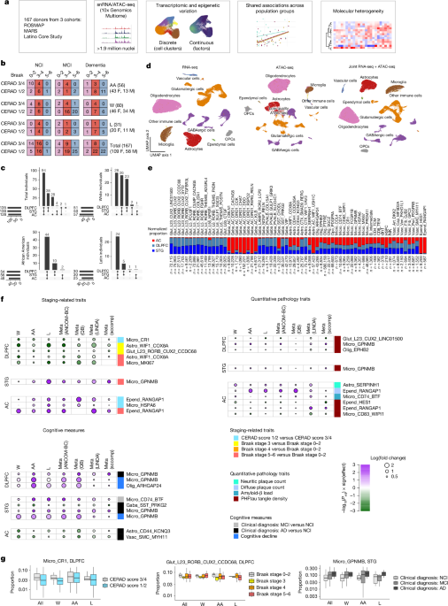
All brain tissue was obtained from participants in the Religious Order Study and Memory and Aging Project (ROSMAP)¹⁹, the Minority Aging Research Study (MARS)²⁰ and the Latino Core Study²¹. As described previously, all participants are without known dementia at enrolment and have annual clinical evaluations; participants whose brain tissue was profiled in this study also consented to brain donation. At death, the brains undergo a quantitative neuropathological assessment, and the participant’s rate of cognitive decline is calculated from the longitudinal cognitive measures, which include up to 31 yearly evaluations¹⁹. An institutional review board at Rush University Medical Center approved each study, and an institutional review board at Columbia University Irving Medical Center approved the use of the post-mortem tissue samples for molecular analysis. All participants included in the analyses presented here signed an informed consent, Anatomical Gift Act and repository consent. For this study, we selected 167 participants, including all donors from the MARS and Latino Core Study who had full pathological characterization by December 2022, and availability of fresh-frozen tissue from at least two of the three brain regions profiled (DLPFC, STG and AC). As a result, our study cohort includes diverse individuals across the full range of the pathological stages and diagnosis of AD and MCI^41,42,43. A subset of demographic and clinicopathological characteristics are summarized in Fig. 1 and Extended Data Fig. 1. Pathological measures were collected as previously described^44,45. We focused our analysis on the following measures:

1. (1)

   CERAD neuritic plaque score^42,46: a semiquantitative measure of neuritic plaques. A neuropathological diagnosis was made of no AD, possible AD, probable AD or definite AD on the basis of semiquantitative estimates of neuritic plaque density as recommended by CERAD, modified to be implemented without adjustment for age and clinical diagnosis. A CERAD neuropathological diagnosis of AD required moderate (probable AD) or frequent (definite AD) neuritic plaques in one or more neocortical regions. Diagnosis includes algorithm and neuropathologist’s opinion, blinded to age and all clinical data. The coded values correspond to 1 (definite), 2 (probable), 3 (possible) and 4 (no AD).

2. (2)

   Braak stage⁴²: a semiquantitative measure of the severity of neurofibrillary tangle (NFT) pathology. The Bielschowsky silver stain was used to visualize NFTs in the frontal, temporal, parietal and entorhinal cortex, and the hippocampus. Braak stages were based on the distribution and severity of NFT pathology: Braak stages 1 and 2 indicate NFTs confined mainly to the entorhinal region of the brain; Braak stages 3 and 4 indicate the involvement of limbic regions such as the hippocampus; and Braak stages 5 and 6 indicate moderate to severe neocortical involvement. Diagnosis includes algorithm and neuropathologist’s opinion.

3. (3)

   Neuritic plaque counts: a quantified measure determined by microscopic examination of silver-stained slides from five regions: midfrontal cortex, midtemporal cortex, inferior parietal cortex, entorhinal cortex and hippocampus. The count of each region is scaled by dividing by the corresponding standard deviation. The five scaled regional measures are then averaged to obtain a summary measure for neuritic plaque counts.

4. (4)

   Diffuse plaque counts: a quantitative measure determined by microscopic examination of silver-stained slides from five regions: midfrontal cortex, midtemporal cortex, inferior parietal cortex, entorhinal cortex and hippocampus. The count of each region is scaled by dividing by the corresponding standard deviation. The five scaled regional measures are then averaged to obtain a summary measure for diffuse plaque counts.

5. (5)

   Amyloid-β load⁴⁷: a quantified measure of amyloid-β protein identified by molecularly specific immunohistochemistry and quantified by image analysis. The value is the percentage area of cortex occupied by amyloid-β, and the overall score is the mean score in eight regions (four or more regions per individual are needed to calculate). The square root of this final score was used for association analyses.

6. (6)

   PHFtau tangle density⁴⁷: a quantitative measure of neuronal NFTs, identified by molecularly specific immunohistochemistry (antibodies to abnormally phosphorylated tau protein, AT8). Cortical density (per mm²) is determined using systematic sampling. Mean of tangle score in eight regions (four or more regions are needed to calculate). The square root of this final score was used for association analyses.

7. (7)

   Clinical diagnosis⁴⁸: physician’s overall cognitive diagnostic category, based on all available clinical data at the time of death. All available clinical data were reviewed by a neurologist with expertise in dementia, and a summary diagnostic opinion was rendered on the most likely clinical diagnosis at the time of death. Summary diagnoses were made blinded to all post-mortem data. Case conferences including one or more neurologists were used for consensus on selected cases. For this study, the categories used were NCI (no cognitive impairment; no impaired domain), MCI (mild cognitive impairment; one impaired domain) and Alzheimer’s dementia.

8. (8)

   Slope of cognitive decline: a quantitative measure based on uniform structured clinical evaluations—including a comprehensive cognitive assessment—that are administered annually to the participants and have been summarized in previous publications^49,50. Scores from 19 cognitive performance tests, 17 of which were used to obtain a summary measure for global cognition, as well as measures for 5 cognitive domains of episodic memory, visuospatial ability, perceptual speed, semantic memory and working memory. The summary measure for global cognition is calculated by averaging the standardized scores of the 17 tests, and the summary measure for each domain is calculated similarly by averaging the standardized scores of the tests specific to that domain. To obtain a measurement of cognitive decline, the annual global cognitive scores are modelled longitudinally with a mixed-effects model, adjusting for age, sex and education, providing person-specific random slopes of decline (which we refer to as the slope of cognitive decline). For association analyses in this study, the negative of the slope value was used (so that higher values of the association variable correspond to steeper slopes of decline).

Generation of snRNA-seq and snATAC-seq (multiome) data

Tissue preparation

This study profiles post-mortem frozen human brain tissue isolated from the DLPFC (BA9), SPG (BA22) and AC, from individuals in the ROSMAP, MARS and Latino Core Study cohorts at Rush University. Tissue from each of these regions was dissected while frozen from flash-frozen tissue blocks at Rush University and sent to Columbia University. Working on ice throughout, we dissected out the white matter and meninges, when present. The following steps were also performed on ice: about 50–100 mg of grey-matter tissue was transferred into a Dounce homogenizer (Sigma, D8938) with 2 ml NP40 lysis buffer (0.1% NP40, 10 mM Tris, 146 mM NaCl, 1 mM CaCl₂, 21 mM MgCl₂ and 40 U ml⁻¹ of RNAse inhibitor (Takara, 2313B)). Tissue was gently dounced while on ice 25 times with pestle A followed by 25 times with pestle B, then transferred to a 15-ml conical tube. Next, 3 ml of phosphate-buffered saline (PBS) + 0.01% bovine serum albumin (BSA) (NEB, B9000S) and 40 U ml⁻¹ of RNAse inhibitor were added for a final volume of 5 ml and then immediately centrifuged with a swing bucket rotor at 500g for 5 min at 4 °C. Samples were processed two at a time, the supernatant was removed and the pellets were set on ice to rest while processing the remaining tissues to complete a batch of three samples for each run of the 10x Genomics Chromium platform (see pooling information below and in ‘Data availability’). The nuclei pellets were then resuspended in 500 ml of PBS + 0.01% BSA and 40 U ml⁻¹ RNAse inhibitor. Nuclei were filtered through 20-μm pre-separation filters (Miltenyi, 130-101-812) and counted using the Nexcelom Cellometer Vision and AO/PI stain at a 1:1 dilution with a cellometer cell counting chamber (Nexcelom, CHT4-SD100-002).

Library preparation and sequencing

To generate snRNA-seq + snATAC-seq (multiome) data, individual samples were pooled into groups of three, with each pool containing (as far as possible) one sample from each of the three regions, and balanced across population groups to minimize batch effects (https://www.synapse.org/Synapse:syn53649030). Approximately 20,000 total nuclei from three samples were pooled into a single sample and these nuclei were run on the 10x Genomics Chromium platform using the 10x multiome protocol (Chromium Next GEM Single Cell Multiome ATAC + Gene Expression Reagent Bundle, PN-1000283). In brief, after transposition, gel beads-in-emulsion (GEMs) were generated by combining barcoded gel beads, transposed nuclei, a master mix that includes reverse transcription (RT) reagents and partitioning oil on a Chromium Next GEM Chip J (10x Genomics; PN-2000264). Incubation of the GEMs in a thermal cycler for 45 min at 37 °C and for 30 min at 25 °C generated full-length cDNA from poly-adenylated mRNA for the gene-expression library and a Spacer sequence that enabled the attachment of barcodes to transposed DNA fragments for the ATAC library. This was followed by a quenching step that stopped the reaction. Next, GEMs were broken, and pooled fractions were recovered. Silane magnetic beads were used to purify the first-strand cDNA from the post-GEM–RT reaction mixture. Barcoded transposed DNA and barcoded full-length cDNA from poly-adenylated mRNA were pre-amplified by PCR and the products were used as input for both ATAC library construction and cDNA amplification for gene-expression library construction. Libraries were pooled and sequenced together on a NovaSeq 6000 with an S4 flow cell (Illumina) at the New York Genome Center, for a target coverage of around 645 million reads per sample for snRNA-seq and 645 million reads per sample for ATAC-seq. The snATAC-seq libraries were sequenced as follows: read 1N, 50 cycles; i7 index, 8 cycles; i5 index, 24 cycles; read 2N, 49 cycles. The snRNA-seq libraries were sequenced as follows: read 1, 28 cycles; i7 index, 10 cycles; i5 index, 10 cycles; read 2, 90 cycles.

Primary processing of sequencing data

Raw fastq files were aligned to the genome or transcriptome and quantified using the CellRanger ARC v.2.0.2 package (https://www.10xgenomics.com/support/software/cell-ranger-arc/downloads) with default parameters. snRNA-seq count files were then processed with the CellBender package v.0.2.0⁵¹ (https://github.com/broadinstitute/CellBender) to remove background signal, also with default parameters. The post-processing CellBender h5 files were then used for downstream analysis and demultiplexing.

Demultiplexing of sample barcodes and assignment to donors

Because each multiome library consisted of nuclei from three samples from different donors, the original donor of nuclei contained in each droplet was inferred through single-nucleotide polymorphisms (SNPs) in snRNA-seq reads using the freemuxlet workflow in the popscle package⁵² (http://github.com/statgen/popscle). The pooling of samples was designed such that no pair of individuals was represented in more than one library—this design allowed us to demultiplex and assign nuclei to individuals even without their reference genotype information (multiplexing plan included in the data deposited; see ‘Data availability’). Freemuxlet was run on each 10x Genomics run, with the assumption of three donors (each contributing one sample) in the mixture of nuclei. Finally, the donor-specific VCFs generated by freemuxlet were compared across all batches, allowing us to assign each donor group a unique identity based on the combination of batches it appears in. We then assigned each singlet nucleus to the original donor.

Clustering of nuclei

To assign nuclei to individual clusters, we focused on the snRNA-seq data, and clustered nuclei using the Seurat v.4 package⁵³ (https://satijalab.org/seurat/) from each 10x Genomics batch separately to identify major cell classes: glutamatergic neurons, GABAergic neurons, oligodendrocytes, oligodendrocyte precursor cells (OPCs), microglia, astrocytes, vascular cells, ependymal cells and non-microglial immune cells. Only nuclei with more than 500 UMIs (based on snRNA-seq) and a mitochondrial UMI percentage lower than 5% were retained. We then aggregated nuclei from each of these broad classes from all batches, and subsequently subclustered each broad class separately; this included four rounds in which clusters with mixed signatures were iteratively removed. After data clean-up, nuclei from each broad cell type were clustered over a range of PCs and resolution parameter values, and an optimal clustering was selected on the basis of the Calinski–Harabasz and Davies–Bouldin scores. To assign nomenclature to each cluster, we examined the fraction of expression of each gene and each cluster, and selected the most differential genes, some in combination, to uniquely identify each cluster. The final parameters for each broad cell type were as follows: astrocytes (10 PCs, resolution 0.3); ependymal cells (10 PCs, resolution 0.05); GABAergic neurons (10 PCs, resolution 0.4); glutamatergic neurons (10 PCs, resolution 0.4); microglia (20 PCs, resolution 0.2); oligodendrocytes (10 PCs, resolution 0.05); OPCs (10 PCs, resolution 0.05); vascular cells (10 PCs, resolution = 0.1). After each broad cell type was clustered, subclusters were merged if they did not have at least four genes with abs(log₂-fold change) > 2 in each direction for every pair of subclusters. For non-microglial immune cells, cells were not clustered, but rather mapped to the HuBMAP Azimuth annotation using the existing interface (https://azimuth.hubmapconsortium.org/). After quality control, iterative clean-up and removal of nuclei with ambiguous or doublet donor assignments, we retained 1,914,581 nuclei for downstream analysis, out of an initial set of 2,967,275 nuclei.

Associations of cell-type proportions with clinical and pathological traits

To identify statistically significant differences in cluster proportions across various pathological and clinical conditions, we used four methods: three published methods (ANCOM-BC⁵⁴, LINDA⁵⁵ and sccomp⁵⁶) and a quasibinomial regression approach to assess differences in cell cluster proportions (described in more detail below). P values and effect sizes plotted in Figs. 1 and 2 are all from ANCOM-BC, with the corresponding values for the other models reported in Supplementary Table 1. For the published methods, we used standard workflows with default settings for all parameters. For the quasibinomial model, we took advantage of the fact that relative cell-type proportions are naturally distributed in the closed interval [0–1]. Therefore, we used logistic regression with a logit link to model response variables in that interval. However, compositional data tend to be enriched with zeroes, depleted of ones and left-skewed. We modelled this with a quasibinomial distribution that uses an extra parameter to account for overdispersion. We also accounted for heteroskedastic residuals using robust standard errors calculated with White’s original method using the R package sandwich. Using the R package performance, we assessed the model assumptions and the influence of outliers. We computed the 95% confidence intervals based on these robust standard errors using the R package broom. Finally, for each model, we ran multiple iterations randomizing the relative cell-type proportions across participants to assess model calibration and the rate of false positives.

For all methods, we modelled only cell types with at least one more observation than the total number of terms in the models being run: “proportion ~ variable_of_interest + age_at_death + sex + pmi” (where pmi denotes post-mortem interval in hours) for pathological traits and “proportion ~ variable_of_interest + age_at_death + sex + pmi + education” for cognitive traits. Cell compositional analyses were done separately for each broad class: glutamatergic neurons (DLPFC and STG only), GABAergic neurons (including only the relevant GABAergic types in each region), microglia, astrocytes, oligodendrocytes and vascular cells. OPCs were not tested, because they did not have any discrete subclusters, and non-microglial immune cells were also excluded, because of low cell numbers.

Finally, for the cell cluster association analysis in the DLPFC replication datasets^6,8, we used ANCOM-BC on both the original reference cluster calls and the mapped cluster names, with the same associated variables and covariates as in our dataset.

Meta-analysis across populations

To identify consistent signals across the three population groups, we modelled each group independently and then meta-analysed. For all of our proportion analyses (ANCOM-BC, LINDA, sccomp and the quasibinomial model), we used the package metafor to run a meta-analysis using maximum likelihood or a fixed-effects model with a t-test for the coefficients. For a given compositional analysis method, all meta-analysis P values were adjusted using the Benjamini–Hochberg method to obtain FDR-adjusted P values; these corrections were implemented for each broad cell class, over all combinations of cell cluster (minimum 4, maximum 15) × clinical or pathological trait (11) × region (minimum 2, maximum 3), resulting in batches of 88 to 495 P values being adjusted at the same time. We determined that a specific cell-type–phenotype association was shared across all three population groups only if (1) the FDR-adjusted P value was less than 0.1; (2) the sign of association was the same in all groups; and (3) the meta-analysis I² value was lower than 50%. These criteria had to be met for at least two of the compositional methods (ANCOM-BC, LINDA, sccomp and the quasibinomial model) with the same directionality of effect.

Identifying cell-type factors through scHPF

To identify factors modelling continuous gene-expression variation, we used the scHPF method²⁵ to generate factors within each broad cell class. For GABAergic neurons, we calculated factors separately for the AC and for the cortex (both regions aggregated). For glutamatergic neurons, we calculated factors only for the cortex, given the paucity of glutamatergic neurons in the caudate. For each run of scHPF on each broad cell class, we identified the optimal number of factors by selecting the largest factor set such that no two factors had a gene-weight vector or cell-weight vector correlation greater than 0.75. For the selection of genes to represent each factor for visualization, we selected the five genes with the largest weights, as well as a mean pseudobulked counts per million (CPM) > 10 across all nuclei in the broad class of interest.

For factor associations with AD phenotypes, we calculated the median factor value per donor–region combination, and ran simple linear models with the same general covariates as in the proportion analyses described above: “proportion ~ variable_of_interest + age_at_death + sex + pmi” for pathological phenotypes and “proportion ~ variable_of_interest + age_at_death + sex + pmi + education” for phenotypes that include assessments of cognition. As with the compositional analysis, we ran a fixed-effects meta-analysis across the population groups, adjusted P values within each broad class (across all clinical and pathological traits and regions) using the Benjamini–Hochberg method, and report as significant only the factor–trait combinations that passed the following criteria: (1) FDR-adjusted meta-analysis P < 0.1; (2) sign of association the same in all population groups; and (3) meta-analysis I² < 50%.

WGCNA

As well as identifying factors using scHPF, we also performed WGCNA²⁶, as an alternative method to characterize associations between modules of genes and clinicopathological phenotypes. We used the R package WGCNA v.1.74-5, starting with pseudobulked data (CPM) aggregated per donor and region for seven broad classes of cells. Within each class, we retained only genes with CPM > 10 in at least 5 samples, and identified cell-type-specific soft-threshold powers on the log-transformed CPM matrices: glutamatergic neurons (power = 10), AC GABAergic neurons (power = 12), cortical GABAergic neurons (power = 10), astrocytes (power = 4), oligodendrocytes (power = 6), OPCs (power = 4), microglia (power = 4) and vascular cells (power = 3). All signed modules for each cell type were generated using the blockwiseModules function with default parameters, except for the following: deepSplit=2, minModuleSize=30, maxBlockSize=80000, reassignThreshold=0 and mergeCutHeight=0.3.

After identifying gene modules for each cell type, we assessed the enrichment of each module’s genes with cluster differential genes and gene factor loadings. We used the fgsea package in R to calculate P values of enrichment of the genes in a given module in the ranked list of cluster differential genes (for each discrete cluster) and in the ranked list of factor loadings (for each scHPF factor).

All module association analyses with pathological and clinical measures were run in the same way as for the scHPF factors as described above, except that module eigengenes per sample were used instead of median factor values. This includes the same approach for multiple testing correction, and the same criteria for evaluation for meta-analysis P values. However, we also included one additional criterion for significance of modules with traits: all meta-analysis P values had to be more significant than the lowest P value for module 0 eigengene for each cell type. Because module 0 in each cell type does not represent a coherent set of correlated genes, it can be used as a bound to eliminate potential false positives.

Gene ontology analysis

For enrichment analysis, differentially upregulated genes were identified for each subcluster relative to all other subclusters of the same major cell class using the standard edgeR package workflow, with counts pseudobulked per individual sample (donor + region). Genes were first filtered to include only those with at least 10 CPM in at least 10 pseudobulked samples for the cluster of interest. Genes for enrichment were selected according to the following criteria: (1) Benjamini–Hochberg FDR-adjusted P < 0.05; (2) mean pseudobulk CPM ≥ 10 for the cluster of interest; and (3) at least twofold higher expression (log₂-fold change > 1) in the cluster of interest. Genes that satisfied these criteria were then assessed for ‘biological process’ enrichment using the topGO R package, filtered to those processes with a Fisher’s test P_adj < 0.1 and aggregated into broader categories using the rrvrgo package.

For factors, genes were filtered to include only those detected in 5% of pseudobulked samples in a given cell class, and with a mean CPM > 5 across all pseudobulked samples. Of these genes, the top 100 were selected for each factor on the basis of their loading scores, and were fed directly into the topGO package for biological process enrichment. Aggregation and visualization were done in the same way as for cell clusters, using the rrvrgo package with pathways selected on the basis of a Fisher’s test P_adj < 0.1.

snATAC-seq visualization and differential peak analysis

snATAC-seq peaks were first calculated separately for each batch using CellRanger ARC v.2, as described above. Peaks were then aggregated separately across major RNA-defined cell classes (glutamatergic neurons, GABAergic neurons, astrocytes, oligodendrocytes, OPCs, vascular cells, microglia and other immune cells) after the RNA quality control steps outlined above; this resulted in a different set of peak regions called for each major cell class. Peak aggregation and harmonization across samples within each cell class was done using the Signac library in Seurat. Clustering of nuclei in each major cell class using snATAC-seq data was performed within each RNA-defined major cell class using the standard workflow in Signac (latent semantic indexing for dimensionality reduction, followed by Louvain community detection), but did not identify robust subclusters from the Calinski–Harabasz and Davies–Bouldin indices, so no snATAC-seq subclusters were called. Uniform manifold approximation and projection (UMAP) visualizations for ATAC-seq data and for joint snRNA-seq and ATAC-seq data were performed on a subset of 300,000 nuclei randomly sampled across all populations; peaks were harmonized across all nuclei regardless of major cell class. UMAPs for snRNA-seq were based on principal component analysis for dimensionality reduction (30 PCs used); UMAPs for ATAC-seq were based on latent semantic indexing for dimensionality reduction after harmonizing peak calls across the 300,000 nuclei; and UMAPs for joint snRNA-seq and snATAC-seq were based on joint clustering using the WNN workflow in the Signac⁵⁷ R package.

Differential snATAC-seq occupancy among RNA-defined subclusters was measured using the DESeq2⁵⁸ R package on pseudobulked snATAC-seq data. Pseudobulk counts were generated by summing counts for all peak regions within each donor + region sample for that subcluster, after harmonization of peaks within each major cell class. DESeq2 was run for each subcluster (against pseudobulked samples from all other subclusters within the same major cell class) with batch, donor post-mortem interval and donor age at death as covariates. All P values were adjusted using the Benjamini–Hochberg FDR correction. For visualizing the top two peaks per subcluster (Fig. 3a), peaks were sorted by P value, and the top two peaks with positive log₂-transformed fold change were selected.

For transcription-factor-binding site and motif enrichment analysis (Fig. 3b), all cluster-specific differential peaks with FDR-adjusted P < 0.05 and positive log₂-transformed fold changes were inputted into the XSTREME algorithm in the MEME suite using the interactive submission mode (https://meme-suite.org/meme/doc/xstreme.html). Transcription factors with enriched binding sites in each subcluster were then selected after filtering out sequence motifs with more than eight repetitions of the same nucleotide and filtering out sequences found in more than one subcluster.

Open chromatin quantification for AD risk loci

snATAC-seq peak counts were pseudobulked as described above, but for all nuclei from a donor + region sample belonging to each major cell class (instead of each subcluster, as in the description above). Pseudobulked values were then normalized to CPM within each donor + region + cell class sample. For each AD risk locus, CPM counts for all peaks overlapping with the locus (even partially, at the start and end points of the locus) were summed together for each sample. To allow for relative differences in peak locations and widths across different major cell class, these summed CPM values were then divided by the total length of peak regions, and then the mean length-normalized CPM value was calculated for each population group for all samples of a given region and major cell class. Finally, for plotting, the population mean length-normalized CPM value for each locus was divided by the maximum value (across all major cell classes and population groups). The values presented in Fig. 3c therefore underwent four transformations: (1) sample-specific normalization for total read count; (2) length normalization to account for total peak length within a locus; (3) mean calculation and aggregation for each of our three population groups; and (4) normalization to the maximum value for a given locus, to allow for visualization of loci simultaneously.

To assess differential peak occupancy across population groups in each broad cell class, we performed a Kruskal–Wallis non-parametric test on donor-level pseudobulked CPM values for each locus (Supplementary Table 10). Raw P values were adjusted for multiple testing within each broad cell class using the Bonferroni correction. Post-hoc pairwise test P values were then calculated using Mann–Whitney non-parametric tests between population groups; these post-hoc values were not further adjusted.

Xenium multiplexed ISH experiments

The Xenium In Situ technology uses targeted panels to detect gene expression. Here, we used a custom gene list based on cell cluster markers from snRNA-seq (for a full list of genes on the panel see Supplementary Table 2). The probes were designed to contain two complementary sequences that hybridize to the target RNA and a third region encoding a gene-specific barcode so that the paired ends of the probe bind to the target RNA and ligate to generate a circular DNA probe. If the probe experiences an off-target binding event, ligation should not occur, suppressing off-target signals and ensuring high specificity. The Xenium workflow (using in-development chemistry and a prototype instrument and consumables) began by sectioning 10-μm fresh-frozen tissue sections onto a Xenium slide, followed by permeabilization to make the mRNA accessible. The mRNAs were targeted by the probes described above and two negative controls: (1) probe controls to assess non-specific binding and (2) genomic DNA controls to ensure that the signal is from RNA. Probe hybridization occurred at 50 °C overnight with a probe concentration of 10 nM. After stringency washing to remove unhybridized probes, probes were ligated at 37 °C for 2 h. During this step, a rolling circle amplification (RCA) primer was also annealed. The circularized probes were then enzymatically amplified (for 1 h at 4 °C followed by 2 h at 37 °C), generating multiple copies of the gene-specific barcode for each RNA-binding event, resulting in a strong signal-to-noise ratio. After washing, background fluorescence was quenched chemically. The biochemistry is designed to mitigate autofluorescence, which is a known issue owing to the presence of lipofuscins, elastin, collagen and red blood cells, and owing to formalin fixation itself. Sections were placed into an imaging cassette to be loaded onto the Xenium Analyzer instrument. The Xenium Analyzer is fully automated and includes an imager (imageable area of about 12 × 24 mm per slide), sample handling, liquid handling, wide-field epifluorescence imaging, capacity for two slides per run and an on-instrument analysis pipeline. The imager is a fast area scan camera featuring a high numerical aperture, a low read noise sensor and approximately 200 nm per pixel resolution. On the Xenium Analyzer, image acquisition was performed in cycles. The reagents, including fluorescently labelled probes for detecting RNA, were automatically cycled in, incubated, imaged and removed by the instrument. After the binding of fluorescent oligos to the amplified barcode sequence, the sample underwent 15 rounds of fluorescent probe hybridization, imaging and probe removal. The z-stacks were taken with a 0.75-μm step size across the entire tissue thickness. The Xenium Analyzer captured a z-stack of images every cycle and in every channel, which needed to be processed and stitched to build a spatial map of the transcripts across the tissue section. Stitching was performed on the DAPI image, taking all of the stacks from different fields of view (FOVs) and colours to create a complete three-dimensional (3D) morphology image (morphology.ome.tif) for each of the stained regions. First, the lens distortion in internal sensor data was corrected on the basis of instrument calibration data, which were collected to characterize the optical system and were saved on the instrument. Next, the z-stacks from the internal sensor data were further subsampled to a 3-μm step size, which was determined empirically to be a useful resolution for cell segmentation quality. Image features were then extracted from the regions where FOVs overlapped. Feature matching was performed to estimate the offsets between adjoining FOVs. The offsets were used to ensure consistent global alignment across the image. Finally, the 3D DAPI image volumes (z-stacks) generated across FOVs were stitched together. RCA product image processing was then applied to detect and filter puncta and correct distortion. A punctum is a point source in microscopy that is smaller than a pixel and is measured in units of observed photons. The 3D image volumes (z-stacks) obtained for each FOV were processed, for 4 colour channels and 15 cycles, to detect the puncta in 3D space that correspond to labelled RCA products. The RNA fluorescence images were scanned for punctum signals that stood out from the local background. The XYZ coordinates of each punctum were refined by examining the local brightness. The signal intensity of the punctum was determined by fitting a Gaussian distribution to the observed emitted light to determine the centre, size and intensity of the point sources. We filtered out puncta that were unlikely to be from true RCA products (non-punctate or low-quality signals). Similar to DAPI images, curvature distortion was corrected. To proceed from puncta to transcripts, decoding was performed using a Xenium codebook—a collection of code words that were assigned to genes in the gene panel. Each code word was defined on the basis of an expected pattern of fluorescent signals recorded across channels and cycles. Some code words were reserved for negative controls. The fluorescent signals from all channels and cycles were compared with the codebook using a global (across all FOVs) maximum likelihood approach. This approach considered attributes such as puncta locations, their colour and cycle of detections and signal intensities. To assign mRNA transcripts to cells, we used the default segmentation parameters in Xenium Onboard Analysis (XOA) v.3.0, which segments cells on the basis of DAPI staining, with an expansion distance of 5 µm or until another cell boundary is encountered.

Analysis of Xenium data

Processing and downstream analysis of the Xenium counts matrix was performed using the Seurat v.5 package in R, as follows:

1. (1)

   For each section, all segmented objects (cells) with fewer than 20 total transcript counts were removed.

2. (2)

   Labels derived from snRNA-seq clusters were then used to generate a set of reference profiles for label transfer. snRNA-seq counts were pseudobulked (raw counts summed) for all clusters per donor for every DLPFC sample (excluding the AC-specific clusters) and pseudobulk profiles with more than 5,000 total counts were retained. These pseudobulked data were then used as the reference for label transfer.

3. (3)

   The RCTD workflow³⁹ was run on the Xenium data, using the pseudobulked snRNA-seq-derived profiles. This workflow, implemented in Seurat v.5, consisted of the spatialRNA, create.RCTD (UMI_min = 20) and run.RCTD (doublet_mode = ”doublet”) commands.

4. (4)

   Transferred labels were assessed by plotting cluster marker expression per cluster (Fig. 4b), with notes made as to which transferred clusters did not show the expected expression of markers.

5. (5)

   For each Xenium sample, all objects within the grey matter were manually assigned by drawing boundaries around the grey matter using the gatepoints package in R. Grey–white matter boundaries were identified using cellular (segmented object) density and expression of MOG and RBFOX3.

6. (6)

   For validation of snRNA-seq-derived proportion analyses, ANCOM-BC was run in the same way as for the snRNA-seq data, but using cell cluster proportions in the grey matter of the Xenium sections.

Mapping cell cluster labels across studies

Cluster calls from this dataset were mapped to nuclei from two previously publisheddatasets^6,8 using the MapMyCells package from the Allen Institute for Brain Science (https://portal.brain-map.org/atlases-and-data/bkp/mapmycells). Nuclei from this study were randomly assigned to five groups, and a separate MapMyCells model was built for each set of nuclei. The nuclei from the query datasets^6,8 were then assigned five cluster labels, one from each of the five models. Nuclei that received the same label from at least four of the five models were assigned that cluster label, and nuclei that did not meet this criterion were called ‘ambiguous’ and not retained for downstream analysis. This same procedure was also run in the other direction, for mapping cluster names from these two datasets (as reference) onto this study (as query).

Donor clustering based on cell subcluster frequencies and median factor scores

To identify potential subgroups of donors on the basis of cell-type profiles, the within-broad-class normalized proportions of astrocyte, neuronal, oligodendrocyte, microglial and vascular clusters, as well as the median factor values per donor, were concatenated into input vectors for hierarchical clustering approach, with 1 − Pearson’s correlation r value as the distance measure and Ward’s method for linkage. The resulting hierarchical tree was cut at various heights, and silhouette scores were calculated at each height. The median silhouette score at each cut height was used to determine that six groupings was optimal. For each of these six groups, the number of donors for each cognitive diagnosis, Braak stage, CERAD score and population group were calculated, as shown in Fig. 5a.

We evaluated whether the clustering partitions acquired using hierarchical clustering with Ward’s D method for linkage and dissimilarity through Spearman correlation were generalizable to (1) minor changes to the initial dataset or (2) the clustering method used. We evaluated the robustness of eight algorithms: three that used different correlation metrics ((1) Pearson, (2) Spearman and (3) Kendall) but which retained the use of hierarchical clustering with Ward’s D, and five that did not use Ward’s D but which retained the calculation of dissimilarity with Spearman correlation ((4) hierarchical clustering with Ward’s D2 method, (5) hierarchical clustering with complete linkage, (6) spectral clustering, (7) k-means clustering and (8) partitioning around medoids (PAM) clustering).

We first tested all eight clustering algorithm variations on the initial, unperturbed datasets (consisting of the 17 agglomerated features) to create reference partitions per method. We then performed two robustness analyses. In the first analysis, we added varying amounts of randomly distributed noise centred around a mean of 0 into the 17 agglomerated features. Noise levels ranged from 0.05 to 1 standard deviations of each feature. We tested 100 bootstrap iterations for each noise level and method, and calculated the Jaccard similarity of each bootstrap iteration to the reference partition for that method to create a distribution of Jaccard similarity scores. Across methods, we found that added noise leads to decreased similarity, which was expected. In the second analysis, we shuffled a percentage of each of the values per column across samples. As expected, a higher shuffling percentage resulted in lower similarity to the reference partition. Across both analyses, the PAM method exhibited the highest Jaccard similarity compared with the base partition. We were interested in whether the reference PAM partition corresponded to cognitive diagnoses, and found similar results to those obtained from the reference Ward D cluster assignments. Finally, to qualitatively evaluate whether the reference PAM partition differed substantially from the reference Ward D partition, we plotted river plots showing cluster assignments between the two partitions. We found a large amount of overlap, because many individuals in the same group in one partition were also grouped together in the other.

Genetic ancestry estimation and modelling

To discern the effects of environment and genetics on the associations between AD traits and our molecular features, we used available WGS data from 151 of our 167 donors. The remaining 16 donors belonged to the white racial and ethnic group; this was the largest group, and thus the results should not be affected by their absence. For the Latin and African American groups, we accessed the gatk-Haplotype-called gvcf files on GRCh38, then used GenomicsDBImport to generate jointly genotyped GenDB files, and finally kept only the varying regions using GenotypeGVCFs to generate multi-sample VCFs per chromosome. We then used bcftools (v.1.23) to select only biallelic SNPs and PLINK (v.1.9.0-b.8) to remove variants with more than 2% missing data, exclude rare variants with a minor allele frequency lower than 1% and exclude individuals with more than 5% of their genotypes missing. In addition, we discarded variants that deviated significantly from Hardy–Weinberg equilibrium (P < 1 × 10⁻⁶). We then merged the PLINK quality-controlled files for the white group (83,222,307 variants) with those for the Latin and African American groups (14,669,023 variants), yielding a final variant count of 12,601,138 unique and shared SNP IDs. Finally, we performed linkage disequilibrium (LD) pruning on the multi-ethnic PLINK files to exclude variants in LD (r² > 0.2) within a 200-SNP window, advancing by 50 SNPs, for a total of 1,355,673 variants.

Using those quality-controlled multi-ethnic variants, we computed genomic PCs using PLINK and ADMIXTURE (v.1.3.0) for 1 < k < 9. Admixture loadings and genomic PCs were plotted against all AD traits to assess their correlations. The first two genomic PCs capture mostly racial and ethnic variation (Extended Data Fig. 3), whereas PCs 3 and 4 show no clear patterning with the variables of interest. For ADMIXTURE, k = 3 showed the biggest changes in log-likelihood, normalized ancestry entropy and minimum pairwise Fst (Extended Data Fig. 3). On the basis of these biological metrics and the complementary numerical optimizations, k = 3 was selected for modelling.

For admixture component-based modelling, we ran the same set of meta-analyses (using all four compositional methods and one factor association approach) using the majority admixture component per individual as the grouping variable, instead of self-reported race and ethnic group. The same criteria were used as described above for multiple testing correction and for assessing the robustness of results across methods.

For genetic PC-based modelling, we included the continuous values for PC1 and PC2 as interaction terms with the clinical or pathological trait of interest in two separate models (one for PC1 and one for PC2). No meta-analysis was needed in this case, but multiple testing correction was performed using the same criteria above. Here, we identified cluster and factor associations with a statistically significant main effect (with the trait of interest, FDR-adjusted P < 0.1) and non-significant interaction effect with the genetic PC (FDR-adjusted P > 0.1). As in our other analyses, cluster associations had to be significant after multiple testing correction in at least two out of four compositional methods.

Polygenic risk scoring

We computed polygenic risk scores per donor using the most recent and well-powered AD summary statistics³⁷ in conjunction with the quality-controlled (but not LD pruned) multi-ethnic PLINK file described in the previous section. To account for variants in LD, we first aggregated variants within 250 kb of the lead variant (nominal P < 1 × 10⁻⁵) with r² > 0.1 using PLINK. The effect of these variants was then summed and averaged to score each donor using PLINK.

Reporting summary

Further information on research design is available in the Nature Portfolio Reporting Summary linked to this article.