Universal transcriptomic hallmarks of mammalian ageing and mortality

Experimental samples

Animals from ITP cohorts

Liver samples of mice from the ITP⁶¹ were acquired from the collections of University of Michigan Medical School (UM), University of Texas (UT) and The Jackson Laboratory (TJL), from animals of the 2015, 2016 and 2017 cohorts^8,62,63,64. Female and male mice, 22 to 23 months old, were euthanized following interventions, including 17-DMAG (30 ppm, as in ref. ⁶²), b-GPA (3,300 ppm, as in ref. ⁶²), minocycline (300 ppm, as in ref. ⁶²), mitoQ (100 ppm, as in ref. ⁶²), rapamycin applied from 20 months (42 ppm, as in ref. ⁶²), canagliflozin (180 ppm, as in ref. ⁸), candesartan cilexetil (30 ppm, as in ref. ⁶⁴), geranylgeranyl acetone (600 ppm, as in ref. ⁶⁴), 17-α-oestradiol applied to males from 20 months (14.4 ppm, as in ref. ⁶⁴), 17-α-oestradiol applied to males from 16 months (14.4 ppm, as in ref. ⁶⁴), MIF098 (240 ppm, as in ref. ⁶⁴), nicotinamide riboside (1,000 ppm, as in ref. ⁶⁴), 1,3-butanediol (100,000 ppm, as in ref. ⁶³), captopril (180 ppm, as in ref. ⁶³), leucine (40,000 ppm, as in ref. ⁶³), PB125 (100 ppm, as in ref. ⁶³), sulindac (5 ppm, as in ref. ⁶³), syringaresinol (300 ppm, as in ref. ⁶³), a combination of rapamycin and acarbose applied from 9 months (14.7 ppm and 1,000 ppm, as in ref. ⁶³), and a combination of rapamycin and acarbose applied from 16 months (14.7 ppm and 1,000 ppm, as in ref. ⁶³). All interventions continued until the mice were euthanized. In addition, livers were taken from control untreated male and female mice euthanized at 4–6 and 22 months of age. All mice were fed ad libitum with the same diet (Purina 5LG6) made in the same commercial diet kitchen (TestDiet). Mice represented genetically heterogeneous UM-HET3 strain, produced by crossing female CByB6F1/J and male C3D2F1/J mice. Therefore, each mouse in the cohort had a unique genetic background but shared the same inbred grandparents (C57BL/6J, BALB/cByJ, C3H/HeJ and DBA/2 J). Mice were housed in plastic ventilated cages under similar environmental conditions in all sites (21–23 °C temperature, 40–60% humidity, 12 h:12 h light:dark cycle). Details of the mouse housing and methods used for health monitoring are provided in refs. ^61,65. All experiments were approved by the Institutional Animal Care and Use Committee of each site (The Jackson Laboratory in Bar Harbor (TJL), the University of Michigan at Ann Arbor (UM), and the University of Texas Health Science Center at San Antonio (UT)).

Klotho-KO mice

Eight-week-old male wild-type mice (C57BL/6J) and Klotho^−/− knockout mice were purchased from CLEA Japan. Mice were housed under specific pathogen-free conditions, at a temperature of 22 ± 2 °C, with a relative humidity of 50 ± 10%, and on a 12 h:12 h light:dark cycle. Mice had free access to tap water and standard chow. The animal protocols were approved by the Tohoku University Institutional Animal Care and Use Committee. The animal procedures performed conform to the NIH guidelines (Guide for the Care and Use of Laboratory Animals).

RNA sequencing

Bulk RNA-seq profiling of mouse tissues

For RNA-seq profiling of liver samples from ITP cohorts, three biological replicates (animals) per sex were utilized for each intervention, except for canagliflozin (seven biological replicates per sex). Additional control samples included 24 old and 6 young mice per sex across different cohorts, resulting in 182 total liver samples (Supplementary Table 1a). For RNA-seq profiling of bulk kidney and gastrocnemius skeletal muscle samples from wild-type and Klotho-KO male mice, 6 biological replicates (animals) per group were utilized for every tissue (24 samples total). Samples selected for sequencing were randomly chosen from available animals within each group. No a priori power calculations were performed; sample sizes were determined by cohort availability and by sample sizes used in similar molecular signature and clock application studies^15,21,54. RNA was extracted with PureLink RNA Mini Kit as described in the protocol and submitted for sequencing. Paired-end sequencing with 150 bp read length was performed on Illumina NovaSeq 6000.

Nuclei extraction from tissues of Klotho-KO mice

Brains and kidneys from one 8-week-old control mouse and one age-matched Klotho-KO animal were collected following cervical dislocation and flash frozen in liquid nitrogen. The cortical region of brain and a radial section of the kidney were dissected. Their nuclei were isolated with the Minute single nucleus isolation kit for neuronal tissue/cells and the Minute single nucleus isolation kit for tissue/cells (BN-020, SN-047, Invent Biotechnologies), following the manufacturer’s protocol with minor modifications. Specifically, the isolated nuclei were resuspended in 5% BSA solution with RNase inhibitor (1000494; 10X Genomics).

snRNA-seq profiling of Klotho-KO mouse tissues

snRNA-seq was performed with Chromium Single Cell 5′ Reagent Kits (PN-1000265; 10X Genomics) according to the manufacturer’s instructions. In brief, single-cell suspensions from the tissues were loaded into a Chromium Next GEM Chip K Single Cell Kit (PN-1000287; 10X Genomics), and a Chromium Controller was used for barcoding and cDNA synthesis. A Chromium Next GEM Single Cell 5′ Library & Gel Bead Kit v2 (PN-1000265; 10X Genomics) was used to amplify the cDNA and construct the cDNA libraries. RNA-seq was performed by DNAFORM.

Datasets and external resources

Transcriptomic data for rodent meta-dataset

Mouse and rat gene expression data for meta-analysis and clock development were obtained from the current study (ITP cohorts), published studies^66,67,68 and the repositories NCBI Gene Expression Omnibus (GEO)⁶⁹, ArrayExpress⁷⁰, and Sequence Read Archive (SRA)⁷¹ via the following identifiers: GSE3150⁷², GSE6591⁷³, GSE11291⁷⁴, GSE34378⁷⁵, GSE27625⁷⁶, GSE53960⁷⁷, GSE66715⁷⁸, GSE132040⁷⁹, GSE146977⁸⁰, GSE145480⁸¹, GSE3129⁷², GSE55272⁸², GSE131754¹⁵, GSE81959⁸³, GSE36838⁸⁴, GSE46895⁸⁵, GSE51108⁸⁶, GSE26267⁸⁷, GSE92486⁸⁸, GSE124772⁸⁹, GSE101657⁹⁰, GSE117188⁹¹, GSE32609², GSE1093⁹², GSE40977⁹³, GSE48333⁹⁴, GSE48331⁹⁴, GSE49000⁹⁵, GSE97074⁹⁶, GSE108379⁹⁷, GSE122116⁹⁸, GSE121395⁹⁹, GSE122080¹⁰⁰, GSE122085⁹⁸, GSE122243¹⁰¹, GSE122367¹⁰², GSE126814¹⁰³, GSE127758⁵⁸, GSE128724¹⁰², GSE129083¹⁰⁴, GSE137504¹⁰⁵, GSE139204¹⁰⁶, GSE140286¹⁰⁷, GSE143304¹⁰⁸, GSE145972¹⁰⁹, GSE146796¹¹⁰, GSE147666¹¹¹, GSE148647¹¹², GSE149569¹¹³, GSE155407¹¹⁴, GSE156762¹¹⁵, GSE158980¹¹⁶, GSE165409¹¹⁷, GSE154832¹¹⁸, GSE166615¹¹⁹, GSE166778¹²⁰, GSE168211¹²¹, GSE168610¹²², GSE175571¹²³, GSE178770¹²⁴, GSE69952¹²⁵, GSE78130¹²⁶, GSE83931¹²⁷, GSE93833, GSE124483¹²⁸, GSE127475¹²⁹, GSE190939¹³⁰, GSE201207¹³¹, GSE141252¹³², GSE134781¹³³, GSE134780¹³³, GSE219203¹³⁴, GSE149029¹³⁵, GSE39699¹³⁶, GSE75574¹³⁷, GSE89272¹³⁸, GSE54853¹³⁹, GSE155064¹⁴⁰, GSE86882¹⁴¹, GSE234563¹⁴², GSE51202¹⁴³, GSE84390¹⁴⁴, GSE123293¹⁴⁵, GSE234667¹⁴⁶, GSE52794¹⁴⁷, GSE241904¹⁴⁸, GSE75192¹²⁶, PRJNA281127¹⁴⁹, PRJNA516151¹⁵⁰, E-MTAB-3374¹⁵¹, E-MEXP-2320¹⁵² and E-MEXP-153¹⁵³. The complete annotation of the rodent meta-dataset is in Supplementary Table 1b.

Transcriptomic data for primate meta-dataset

For multi-species meta-analysis and clock development, rodent data were further expanded with two primate species: crab-eating macaque (Macaca fascucularis) and human (Homo sapiens). Gene expression data from more than 30 macaque tissues were derived from the CRA012195¹⁵⁴ dataset (Genome Sequencing Archive (GSA)), and human blood, brain, skeletal muscle and skin gene expression data were obtained from MESA¹⁵⁵ and the following GEO datasets: GSE103232¹²⁶, GSE113957¹⁵⁶, GSE123658, GSE134080¹⁵⁷, GSE17612¹⁵⁸, GSE183701¹⁵⁹, GSE190125¹⁶⁰, GSE21935¹⁶¹, GSE221178¹⁶², GSE226189¹⁶³, GSE36192¹⁶⁴, GSE40645¹⁶⁵, GSE5086¹⁶⁶, GSE53890¹⁶⁷, GSE674¹⁶⁸ and GSE75337¹²⁶. MESA data were derived from dbGaP using accession number phs001416.v3.p1. Controlled-access human data were accessed, processed, and analysed only by dbGaP-approved users, in accordance with the NIH dbGaP Data Use Certification. These data were not transferred outside the approved institutional access framework. The complete annotation of primate transcriptomic meta-dataset is in Supplementary Table 1c.

Bulk gene expression datasets for clock applications

Transcriptomic clocks were applied to multiple independent experimental models of ageing modulation, stress induction, molecular age deceleration, and disease:

• FACS-sorted cell types from young (2-month-old) and old (22–24-month-old) female C57BL/6 mice (GSE223049¹⁶⁹).

• LPS or PBS injection into the brain of 5–6-month-old male and female C57BL/6J mice (GSE250279¹⁷⁰).

• Liver samples from control C57BL/6J, DBA/2J, and C3B6F1 mice and strain-, sex-, and age-matched animals subjected to caloric restriction (GSE92486⁸⁸, GSE81959⁸³, GSE40977⁹³, GSE46895⁸⁵ and GSE49000⁹⁵).

• Kidney and skeletal muscle samples from Klotho-KO progeroid 8-week-old male mice and age-matched C57BL/6J controls (current study).

• Culturing of primary human fibroblasts and their exposure to oligomycin and 2-DG (GSE179848¹⁷¹).

• Culturing of control and hTERT-transduced WI-38 cells (GSE175533¹⁷²).

• OSKM-induced cellular reprogramming of primary human fibroblasts (E-MTAB-3037¹⁷³).

• γ-irradiation (20 Gy) of embryonic (EF) and skin fibroblasts (SF) from mice and naked mole rats¹⁷⁴.

• Liver samples from young (3-month-old) and old (20-month-old) C57BL/6J mice subjected to isochronic or heterochronic parabiosis (GSE224378⁵⁴).

• C57BL/6J mouse embryos at different stages of development, from fertilized eggs to newborn mice (GSE39897¹⁷⁵).

• Tissue samples from healthy C57BL/6, B6SJLF1/J, 129S6/SvEv and B6C3F1 mice and Wistar rats, and strain- and age-matched animals with chronic disease models, including Alzheimer’s Disease 5xFAD model, ischaemic stroke, HCC, CKD, diabetic nephropathy and nonalcoholic steatohepatitis (GSE142633¹⁷⁶, GSE137482¹⁷⁷, GSE148350¹⁷⁸, GSE129586¹⁷⁶, GSE102558¹⁷⁹, GSE189377¹⁸⁰, GSE197699¹⁸¹, GSE120977¹⁸², GSE26538¹⁸³).

• Tissue samples from healthy human participants and those with chronic diseases, including Crohn’s disease, ulcerative colitis, CKD, Alzheimer’s disease and heart failure (GSE135055¹⁸⁴, GSE104704¹⁸⁵, GSE166925¹⁸⁶, GSE157712¹⁸⁷).

scRNA-seq and snRNA-seq datasets

To evaluate ageing and mortality dynamics at single-cell resolution we utilized:

• Droplet Tabula Muris Senis scRNA-seq dataset (GSE149590¹⁸⁸), which covers gene expression profiles of single cells from multiple organs extracted from C57BL/6J mice of different ages, ranging from 1 to 30 months.

• Early C57BL/6 mouse organogenesis (from E6.5 to E8.5) scRNA-seq dataset¹⁸⁹.

• Kidney and brain snRNA-seq data from Klotho-KO progeroid 8-week-old male mice and age-matched C57BL/6J controls (current study).

Framingham Heart Study

Blood RNA-seq (n = 3,709) and DNA methylation profiles (n = 1,796) with linked prospective mortality and CVD onset data were obtained from dbGaP (phs000974.v6.p5). Controlled-access human data were accessed, processed, and analysed only by dbGaP-approved users, in accordance with the NIH dbGaP Data Use Certification. These data were not transferred outside the approved institutional access framework.

UK Biobank proteomics

Plasma concentrations of GPNMB, CDKN1A, and LGALS3 quantified using Olink Proximity Extension Assay platforms were obtained from the UK Biobank data^190,191 together with the linked demographic and phenotypic records related to patients’ mortality, first disease incidence and risk factors. UK Biobank data were accessed and analysed only by approved users. These data were not transferred outside the approved institutional access framework.

Data preprocessing

Processing of generated bulk RNA-seq data

Reads from both bulk RNA-seq datasets (ITP and Klotho-KO) were mapped to the mouse genome (GRCm39) with STAR (v2.7.11b)¹⁹² and counted via featureCounts (v2.0.6)¹⁹³. To filter out non-expressed genes, we retained genes with ≥10 reads in at least 20% of ITP samples or 25% of samples from Klotho-KO dataset, yielding 13,422 and 15,744 detected genes according to Entrez annotation, respectively. Filtered count matrices were normalized using relative log expression (RLE) normalization¹⁹⁴. For the ITP dataset, sex-specific PCA was used to identify outliers. Samples with PC1 or PC2 values > 1.5× IQR beyond the first or third quartile were excluded. A total of 21 samples were identified as outliers and removed from the ITP data. All interventions remained represented after filtering. Full ITP sample annotation is provided in Supplementary Table 1a.

Processing of external gene expression data

Preprocessing of all transcriptomic data was performed in R (v4.4.0) and followed our previously established pipeline¹³. In brief, for each bulk RNA-seq dataset, raw counts were downloaded, soft-filtered to remove unexpressed genes, mapped to the mouse Entrez IDs, RLE-normalized, log-transformed, and scaled. Microarray data were log-transformed, mapped to the mouse Entrez IDs, and scaled. All preprocessing steps were performed separately within each dataset, species, and tissue. Data features were harmonized to mouse Entrez gene identifiers based on 1:1 (mutually exclusive) orthologs identified with biomaRt. For clock development and application, YuGene normalization¹⁹⁵ was also applied as an alternative to scaling because of its robustness for cross-platform integration¹⁹⁶.

Integration of multi-study gene expression data

Preprocessed data were aggregated into a meta-dataset for clock training, signature and module analysis. Genes present in fewer than 20% of datasets were filtered out, yielding 18,592 genes for rodent meta-dataset and 12,897 orthologous genes for multi-species data. For quality control, each sample’s expression profile was correlated (Spearman ρ) with the median profile of matching tissues across the meta-dataset; samples with ρ < 0.5 were removed as outliers. This yielded 3,876 mouse and 663 rat gene expression samples with known chronological age (Supplementary Table 1b), together with 2,623 macaque and 4,003 human tissue samples (Supplementary Table 1c), for a total of 11,165 tissue samples from 4 species.

Relative expression adjustment for batch correction

To minimize technical and biological confounding in the integrated meta-dataset prior to transcriptomic signature analysis and clock development, scaled or YuGene-transformed gene expression profiles were converted into relative log-expression changes. Specifically: (1) within each dataset-tissue combination, a reference group of age-, sex-, and strain-matched control samples was randomly selected; (2) median expression values were computed for each gene across the reference samples; and (3) these medians were subtracted from the corresponding gene expression values of all samples from that dataset and tissue. In parallel, chronological age, normalized age, expected mortality rate (log₁₀(μ)), and expected maximum lifespan were centred by subtracting the corresponding values of the reference group, yielding sample-specific deviations relative to age-matched controls. This relative expression normalization was also used for preprocessing all independent datasets prior to relative clock application.

For transcriptomic signature and module analysis, reference groups were additionally matched by sex, such that centring was performed within dataset-tissue-sex strata to ensure that signatures reflected ageing- and intervention-associated transcriptional changes rather than sex-specific baseline differences in expression. Following calculation of relative expression profiles, outlier samples were identified by PCA and excluded if their scores on the first or second principal component were outside ±1.5× IQR. In addition, genes detected in fewer than 50% of samples were removed prior to all downstream signature analyses.

Processing of Klotho-KO snRNA-seq data

The sequenced snRNA-seq raw data were processed with Cell Ranger (v7.0.0) and Seurat (v5.0.1) package. For quality control, nuclei that were detected with mitochondrial content >10%, <200 genes, or >4,000 genes were considered dying cells, empty droplets and doublets, respectively, and were excluded. Cells were annotated using established marker gene panels for brain and kidney cell types^197,198,199.

snRNA-seq data were normalized, subjected to PCA, and visualized with UMAP separately for each organ with Seurat²⁰⁰. To establish homogeneous clusters of cell types for kidney, we filtered out cells with dimensionally reduced coordinates falling outside the boundaries of the quartiles ±1.5 IQR calculated for the corresponding cell type. Within each annotated cell type, nuclei were aggregated into metacells to achieve a target coverage of ≥200,000 reads per metacell. Metacell data were then processed using the bulk RNA-seq pipeline as described in ‘Processing of external gene expression data’ and centred relative to control samples within each cell type, as described in the ‘Relative expression adjustment for batch correction’.

Processing of scRNA-seq data from Tabula Muris Senis

Raw single-cell gene expression matrices from the Tabula Muris Senis dataset¹⁸⁸ were filtered to retain only tissues represented by at least 7 individual mice and spanning ≥15 months of chronological age, yielding a total of 9 tissues for downstream analysis. Cell-type annotations were obtained from the original dataset metadata.

To enable application of bulk transcriptomic clocks to single-cell data, individual cell expression profiles originating from the same tissue and mouse were aggregated into metacells by summing raw counts across either all available cells or randomly selected subsets of cells per sample (Fig. 2d). Metacell size thresholds ranging from 1 to 750 cells were evaluated to assess the effect of cell number and coverage per metacell on clock performance (Fig. 2e,f). In parallel, to assess tAge of individual cell types, a cell-type-specific aggregation was performed whereby all cells annotated as the same cell type within each individual mouse were pooled into a single metacell.

All metacell expression profiles were subsequently processed using the same pipeline as bulk RNA-seq data (described in ‘Processing of external gene expression data’), including gene filtering, RLE normalization, log transformation and scaling. Relative expression values were computed by centring each expression profile against all metacells within tissue or cell type, as described in ‘Relative expression adjustment for batch correction’.

Processing of early organogenesis scRNA-seq data

Raw count matrices from single-cell RNA-seq data spanning early mouse organogenesis (from E6.5 to E8.5)¹⁸⁹ were processed using a standard droplet-based quality control pipeline. Cells were retained only if they exceeded a minimum threshold of 5,000 unique molecular identifiers and expressed at least 1,000 genes. Cells with high mitochondrial read content (>2.37% of total reads) were excluded. Additional filtering was performed to remove doublets (droplets containing more than one cell) and droplets lacking detectable nuclear RNA signal.

To enable application of bulk transcriptomic clocks to single-cell data, individual expression profiles were aggregated into metacells. For whole-embryo analyses, all cells from each sample were pooled into a single metacell. Metacells with total coverage <200,000 reads were excluded to ensure sufficient sequencing depth for clock application. Aggregated expression profiles were subsequently processed using the same pipeline as bulk RNA-seq data (described in ‘Processing of external gene expression data’). Samples from the earliest presented developmental stage (E6.5) were used as the reference group for relative expression centring.

For lineage-specific clock application, probabilistically weighted metacells were generated based on reconstructed ancestral trajectories (described in ‘Inference of ancestral lineage during early organogenesis’). To ensure sufficient sampling, only cell types represented by ≥400 cells at E8.5 were retained. Additionally, for each cell type, we excluded cells that had zero trajectory membership probability. Then, gene expression counts for each remaining cell were multiplied by their inferred lineage probability (that is, probability of being an ancestor of the corresponding cell type from E8.5). Weighted counts were summed within each sample to generate trajectory-specific metacell profiles, and the resulting values were multiplied by total cell number to preserve read-depth comparability across samples. Only aggregated metacells with total coverage ≥200,000 reads were retained. Resulting metacell profiles were preprocessed using the standard bulk RNA-seq pipeline described in ‘Processing of external gene expression data’, and relative expression values were calculated by centring against E6.5 reference samples prior to clock application.

Analytical methods

Estimation of maximum lifespan, expected mortality, and normalized age

Maximum recorded lifespans for mice, rats, crab-eating macaques and humans (4, 3.8, 39 and 122 years, respectively) were obtained from the AnAge database^201,202. Survival curves for control rodents of different strains and sexes, as well as animals exposed to lifespan-shortening, lifespan-neutral and lifespan-extending interventions, were collected from published studies and digitized when necessary^{2,5,6,7,8,62,63,67,75,82,83,84,85,86,87,89,90,91,94,95,96,97,129,130,133,134,135,136,139,141,142,143,148,152,203,204,205,206,207,208,209,210,211,212,213,214,215,216,217,218,219,220,221,222,223,224,225,226,227,228,229,230}. Survival data for crab-eating macaques were obtained from ref. ²³¹. Human survival data for healthy populations and individuals with Hutchinson–Gilford progeria syndrome, Down syndrome and type I diabetes were derived from US CDC reports²³² and cohort studies^{233,234,235,236,237}.

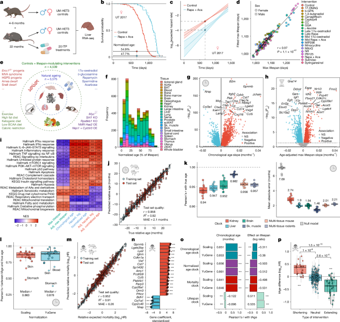
All survival data were fitted with the Gompertz mortality function (adjusted for left truncation) using the flexsurvreg function from flexsurv (v2.3) package²³⁸:

For experimental models (defined by combinations of species, strain, sex and intervention) represented by multiple independent survival curves, aggregated Gompertz parameters were estimated using mixed-effects meta-analysis with restricted maximum likelihood (REML) criterion, implemented via the rma.uni function of the metafor (v4.6-0) package²³⁹, integrating study-level mean and standard error estimates of ln(A) and r.

For every transcriptomic sample included in the analysis the expected hazard rate was calculated via Gompertz model based on the sample’s chronological age and experimental model (species, strain, sex and intervention information). Sample-specific hazard estimates were calculated as the mean of log₁₀(μ) predictions derived from an aggregated mortality model (for the corresponding experimental group) and from the Gompertz model fitted on survival data from the same study when available. For datasets lacking survival information, only aggregated mortality estimates were used.

Gompertz model fitting quality was evaluated by comparing observed 90th percentile lifespans (from survival data) with corresponding estimates from Gompertz-simulated survival distributions. Expected maximum lifespan values (99.9th percentile) for each experimental model (species, strain, sex, and intervention) were obtained from Gompertz-simulated survival curves. Normalized age was calculated as the ratio of chronological age to the expected maximum lifespan (99.9th percentile) simulated for the corresponding experimental model.

Transcriptomic signatures of ageing, mortality and lifespan in the ITP cohort

For the ITP liver RNA-seq dataset, transcriptomic signatures of chronological age, normalized age, expected mortality rate (log₁₀(μ)), and expected maximum lifespan (90th percentile) estimated directly from survival data (‘estimate’) or simulated through corresponding Gompertz models (‘model’), were identified with generalized linear models fitted with edgeR (v4.2.0) package²⁴⁰, with experimental site included as a covariate. Models were fitted separately for males, females, and pooled sexes. For pooled analyses, sex was also integrated in the model as a covariate. Age-adjusted associations with expected mortality, normalized age, and maximum lifespan were assessed by incorporating chronological age as an additional covariate. Statistical significance was determined by Benjamini–Hochberg-adjusted²⁴¹ P < 0.05.

Signature concordance across sexes (Extended Data Fig. 1e) was assessed by calculating Spearman correlations between vectors of gene-specific slope coefficients derived separately for males and females. Associations among pooled-sex signatures across traits were evaluated analogously (Extended Data Fig. 1d). In both analyses, to reduce noise from weakly or non-associated genes, correlations were computed using the union of the top 1,000 most significantly associated genes (with the lowest P values) for each pair of signatures. This denoised signature correlation analysis has been tested and applied previously^13,54,56. Full results of the ITP signature analyses are provided in Supplementary Table 2a–g.

Transcriptomic signatures of ageing, mortality and lifespan in the aggregated meta-dataset

Scaled relative expression profiles from the aggregated meta-dataset were analysed using linear mixed-effects models implemented via lmer from lme4 (v1.1.35.3) and lmerTest (v3.1.3) packages²⁴². Differences in chronological age, normalized age, expected mortality rate (log₁₀(μ)) or maximum (99.9th percentile) lifespan were used as independent variables, while gene log-expression change served as the response variable. Data source and tissue were modelled as random effects, and sex was included as a fixed covariate. Chronological ageing signatures were derived using only untreated control samples. Age-adjusted mortality and lifespan signatures were computed by including chronological age as an additional covariate. Significance thresholds were set at Benjamini–Hochberg-adjusted P < 0.05. Rodent multi-tissue signatures and species-specific ageing multi-tissue signatures are provided in Supplementary Table 2h–n and Supplementary Table 2o–r, respectively.

Pairwise overlaps between transcriptomic signatures associated with different traits were assessed using Fisher’s exact test for upregulated and downregulated genes separately. To evaluate overall similarity between different rodent (Extended Data Fig. 1q) or species-specific signatures (Fig. 2c and Extended Data Fig. 3h,i), each signature was converted into a vector of gene-specific slope coefficients obtained from the mixed-effects models, representing the direction and magnitude of association of each gene with the trait of interest. Pairwise Spearman correlations were then computed between these coefficient vectors, using the union of the top 1,000 most significantly associated genes (with the lowest P values) from each pair of signatures. Thus, individual comparisons involved approximately 1,000–2,000 genes, depending on overlap between signature gene sets.

Top shared ageing-related genes across species (Fig. 2b) were generated using a mixed-effects model (with the metafor package), integrating standardized effect sizes and standard errors from species-specific ageing signatures. Only genes detected across ≥3 species were included. Genes were ranked by standardized aggregated meta-slopes of log-expression. Corresponding P values were adjusted for multiple comparisons using the Benjamini–Hochberg method.

Identification of co-regulated transcriptomic modules of ageing and longevity

To identify clusters of genes that are co-regulated during ageing and in response to lifespan-modulating interventions, WGCNA²⁴³ was applied to the relative scaled rodent and multi-species meta-datasets, centred within dataset, tissue and sex as described above. Samples and genes with excessive missing values were removed with the goodSamplesGenes function, and remaining missing values were imputed using gene-wise medians.

Pairwise Pearson correlations were computed to quantify expression similarity across genes and to construct adjacency matrices using a SoftThreshold = 4. Hierarchical clustering was performed on the resulting topological overlap matrix (TOM) with TOMType = “unsigned”, deepSplit = 2, and minClusterSize = 20, using the dynamic tree cut method. To assess reproducibility of module detection, clustering was also performed independently for rodent males and females (Extended Data Fig. 5a), as well as separately for rodent and primate datasets (Extended Data Fig. 7j). Overlap between modules identified across these analyses was evaluated using Fisher’s exact test.

Initial modules were further refined based on within-module connectivity. Specifically, genes showing weak correlation with the median expression profile of their assigned module were removed. Empirical thresholds for module membership were derived from the maximum Spearman correlation observed in background subsets of 2,500 randomly selected non-module genes, multiplied by a safety factor of 1.1, yielding final cut-offs of ρ > 0.475 for rodent modules and ρ > 0.4 for multi-species modules. This filtering resulted in 28 rodent and 15 multi-species co-regulated gene modules associated with ageing, mortality and lifespan variation.

Functional and upstream regulator enrichment of each module was evaluated using GSEApy²⁴⁴ against Molecular Signatures Database (MSigDB) Hallmark²⁴⁵, KEGG²⁴⁶, Reactome²⁴⁷ and ChEA transcription factor²⁴⁸ ontologies (Supplementary Table 6a,c). Enrichment significance was determined at Benjamini–Hochberg-adjusted P  <  0.05. Based on the top enriched pathways, 26 rodent modules and all 15 multi-species modules were annotated (Supplementary Table 6b,d). These annotated modules were subsequently used for downstream analyses and for development of module-specific transcriptomic clocks.

Module network visualization and association analyses

The rodent gene correlation network was visualized through spectral embedding^249,250 in Python. Pairwise gene correlations were converted to a non-negative adjacency matrix defined as A(i,j) = (cor(i,j), 0). Then, the graph Laplacian (L = D – A) and the random-walk normalized Laplacian L_norm = D^–1L were computed, where D represents the diagonal degree matrix containing weighted node degrees. Eigenvalues and eigenvectors of L_norm were calculated using the eig function from the linalg module in NumPy, and the coefficients of the first and third nontrivial eigenvectors were used as coordinates of a node. For visualization, a subset of 3,000 genes was plotted, including all genes assigned to modules and randomly sampled background genes.

For each module, eigengenes (first principal components) were computed from the rodent relative scaled gene expression meta-dataset. To characterize functional relationships between transcriptomic hallmarks and ageing- or longevity-associated traits, we calculated: (1) partial Spearman correlations between module eigengenes adjusted for chronological age; (2) Spearman correlations between module eigengenes, chronological age, and expected mortality; and (3) partial Spearman correlations between eigengenes and expected maximum lifespan after adjustment for chronological age.

Sparse partial correlation networks were inferred using graphical lasso regularization with model selection based on the extended Bayesian information criterion (EBIC)²⁵¹, implemented using the EBICglasso function from bootnet (v1.6) package²⁵². Resulting Gaussian graphical models were visualized with qgraph (v1.9.8) package using the spring-layout algorithm (Extended Data Fig. 5d). The same approach was used to visualize partial correlation network of predictions obtained from rodent module-specific transcriptomic clocks evaluated on test datasets (Extended Data Fig. 5f,g).

Functional and module enrichment analysis of transcriptomic signatures

Functional and module enrichment were performed for transcriptomic signatures of chronological age, normalized age, expected mortality, maximum lifespan, and individual interventions, including LPS, caloric restriction, Klotho-KO, γ-irradiation, oligomycin, 2-DG, cellular reprogramming, chronic disease models, HPB and embryogenesis. GSEA²⁵³ was applied to pre-ranked gene lists. Genes were ranked using a signed significance score computed as:

where pv is P value reflecting the statistical significance of association between gene expression and the trait or experimental condition of interest, and sgn(slope) indicates the direction of regulation (1 or −1 for positive or negative expression change, respectively).

Gene-level statistics were obtained using dataset-appropriate models: limma²⁵⁴ (v3.60.0) for intervention and disease datasets, edgeR²⁴⁰ (v4.2.0) for ITP cohort analyses, and linear mixed-effects models for aggregated meta-dataset signatures, as described in the corresponding sections.

GSEA was implemented using the fgsea (v1.30.0) package against curated gene sets from the MSigDB, including the Reactome, KEGG and Hallmark collections. For intervention signatures, enrichment was additionally assessed against custom ontologies of transcriptomic module gene sets derived from WGCNA analysis. Rodent module sets were used for interventions in rodent models, and multi-species module sets were applied to interventions in human systems. Statistical significance of pathway and module enrichment was determined using a false discovery rate threshold of 0.05.

Complete lists of significantly enriched pathways and modules for transcriptomic signatures of chronological age, normalized age, expected mortality, and maximum lifespan are provided in Supplementary Table 3, and for intervention signatures in Supplementary Table 7.

For pathway-level signature correlation analysis, Spearman correlation of NES across all gene sets from Reactome, KEGG and Hallmark ontologies was computed for each pair of signatures. For visualization, enriched pathways were hierarchically clustered on NES using complete linkage and Euclidean distance. To reduce redundancy and enhance interpretability, only pathways that were significantly enriched (Benjamini–Hochberg-adjusted P value < 0.05) in at least one signature and represented distinct biological processes were retained for heatmaps.

Inference of ancestral lineage during early organogenesis

Lineage reconstruction during early mouse organogenesis (E6.5–E8.5)¹⁸⁹ was performed using the Waddington optimal transport (WOT) framework²⁵⁵ to infer ancestral probabilities linking cell populations across adjacent developmental stages.

Following quality-controlled preprocessing of single-cell RNA-seq data, the normalization workflow from²⁵⁵ was applied. In brief, total read depth was normalized per cell using counts-per-10,000 (CP10k) scaling (normalize_total function in Scanpy²⁵⁶ v1.9.6 package, with target_sum = 1 × 10⁴), followed by log1p transformation to stabilize variance. Highly variable genes were identified using the highly_variable_genes function (n_top_genes = 3,000), and this gene set was retained for downstream WOT trajectory inference.

To estimate cell growth and death dynamics required for the transport model, z-scores were computed for gene sets associated with cell cycle progression and apoptosis. Individual gene z-scores were truncated to the interval [−5, +5], and mean z-scores across each gene set were calculated per cell using the score_gene_sets function from the wot (v1.0.8.post2) package (with permutations = 0, method = “mean_z_score”), yielding cell-specific birth-death rate estimates. These scores were used to compute growth functions g(x) within the WOT Birth–Death Process model.

Transport matrices linking each pair of adjacent developmental stages were estimated using the OTModel function with parameters ε = 0.05, λ₁ = 1, λ₂ = 50, and growth_iters = 3. To infer ancestral contributions to terminal cell populations at E8.5, cell-type probability vectors were constructed using the population_from_cell_sets function (with at_time = 8.5). These vectors were propagated backward through the transport matrices using the trajectories function in the wot package, generating probabilistic ancestry distributions across all earlier developmental stages.

Reconstructed lineages were validated by two complementary analyses. First, for each E8.5 cell type, dominant ancestral populations were identified at each preceding stage by selecting cell groups cumulatively accounting for ≥90% of total ancestry probability (Extended Data Fig. 10b) and comparing predicted lineages with established developmental relationships. Second, pairwise Spearman correlations were calculated between ancestry probability vectors of all E8.5 cell types to quantify lineage relatedness (Extended Data Fig. 10c), using ancestry distributions cumulatively explaining >99% of total probability for each lineage.

The resulting lineage trajectories were subsequently used to generate probabilistically weighted metacells for lineage-specific transcriptomic clock analyses, as described in ‘Processing of early organogenesis scRNA-seq data’.

Development of transcriptomic clocks

Training data and feature preparation

Transcriptomic clocks were trained on aggregated mouse, rodent, or multi-species meta-datasets comprising tissue gene expression profiles from mice, rats, macaques, and humans (see ‘Integration of multi-study gene expression data’). Scaled or YuGene-transformed expression values were used for absolute clocks, while relative clocks were trained on relative scaled or YuGene-transformed expression profiles centred within dataset-tissue strata, as described in the ‘Relative expression adjustment for batch correction’.

For relative clocks, training features represent gene log-expression deviations from a reference control group drawn from the same dataset and tissue. Corresponding deviations in chronological age, normalized age, expected mortality rate (log₁₀(µ)), and estimated maximum (99.9th percentile) lifespan were used as outcome variables. This approach minimizes batch effects and tissue-specific baseline variability while preserving biologically relevant transcriptomic signals associated with ageing and mortality.

Chronological age clocks were trained exclusively on untreated control samples, whereas clocks of normalized age, expected mortality, and maximum lifespan were trained using both control and intervention-treated samples with defined outcome values. To account for species-specific differences in lifespan, chronological age values were divided by the maximum recorded lifespan of each species (4, 3.8, 39 and 122 years for mice, rats, crab-eating macaques, and humans, respectively^201,202).

For chronological age and normalized age outcomes (scaled to the range from 0 to 1), absolute clocks were trained using either linear or log-log transformed target values:

For development of relative maximum lifespan clocks, two feature configurations were evaluated: models trained using gene expression features alone (as for other clocks), or models trained using gene expression features together with deviations in chronological age included as an additional predictor (Extended Data Fig. 3b).

Supervised machine learning models

Multiple regression algorithms were initially utilized for development of the relative rodent multi-tissue chronological clock, including elastic net, BR, SVM, random forest, KNN and LightGBM. Models were implemented in Python (v3.8.18) using the ElasticNet, BayesianRidge, SVM, RandomForestRegressor and KNeighborsRegressor functions from the scikit-learn library (v1.3.2), and the LGBMRegressor function from the lightgbm package (v4.1.0). Data handling and preprocessing in Python were performed using NumPy (v1.24.4) and pandas (v2.0.3).

Based on cross-dataset stability and predictive accuracy (Extended Data Fig. 2d and Supplementary Table 4a), elastic net and BR models were selected for all subsequent clock development. Elastic net models were used to construct sparse, high-precision clocks with directly interpretable gene coefficients, whereas BR models provided probabilistic point estimates with model-derived standard deviations enabling uncertainty quantification and improved statistical power in smaller datasets. Absolute clocks were developed exclusively using elastic net models, while both elastic net and BR were applied for training relative clocks across tissues and species.

Training procedure and cross-validation strategy

Prior to model fitting, samples were split into training (90%) and held-out test (10%) sets with stratification by species and intervention category (control, lifespan-shortening, neutral, or lifespan-extending). Genes detected in fewer than 20% of training samples were excluded. Missing expression values were imputed using gene-wise medians computed from the training set only, ensuring no information leakage from test samples.

Hyperparameters were optimized using grid search (GridSearchCV) with 5-fold cross-validation (KFold) on the training partitions, maximizing the coefficient of determination (R²). For elastic net models, optimized hyperparameters included alpha (from 10⁻⁵ to 10²) and l1_ratio (from 0 to 1); for BR model, they included initial values for alpha (alpha_init from 10⁻³ to 10⁻¹) and lambda (lambda_init from 10⁻³ to 1); for SVM model they included kernel (linear or rbf), regularization parameter C (from 10⁻⁴ to 1) and epsilon (from 10⁻³ to 1); for KNN they included n_neighbors (from 2 to 10), weights (uniform or distance) and power parameter p (from 1 to 5); for random forest they included n_estimators (from 100 to 2000), max_depth (from 10 to 110), min_samples_split (from 2 to 10) and min_samples_leaf (from 1 to 4); and for LightGBM they included boosting_type (dart or gbdt), num_leaves (from 100 to 250), max_depth (from 1 to 3), n_estimators (from 100 to 5,000), subsample (from 0.5 to 1), min_child_samples (from 50 to 200), min_child_weight (from 10⁻⁵ to 0.1), reg_alpha (from 10⁻⁷ to 1), reg_lambda (from 10⁻⁸ to 1) and colsample_bytree (from 0.2 to 1). Optimal hyperparameters for random forest and LightGBM were identified using randomized search (RandomizedSearchCV) with 60 iterations. Feature centring and scaling (controlled by the with_mean and with_std parameters of StandardScaler) were also included as tunable preprocessing steps and optimized during cross-validation together with model hyperparameters.

Final model selection was performed using grouped fivefold cross-validation (GroupKFold), ensuring that samples from the same experimental dataset did not appear simultaneously in training and validation folds, thereby improving robustness to dataset-specific batch effects and enhancing generalizability to unseen datasets. Final model coefficients for composite elastic net clocks are reported in Supplementary Table 5a. Trained relative composite elastic net and BR clock models are available on Zenodo (https://doi.org/10.5281/zenodo.18763485 (ref. ²⁵⁷)).

Nested cross-validation performance assessment

Clock performance was evaluated on held-out test samples using Pearson correlation (r), coefficient of determination (R²), and MAE metrics. In addition, robust accuracy estimates were obtained through ten iterations of nested cross-validation. In each iteration, samples were randomly divided into training (90%) and testing (10%) subsets. Model training incorporated fivefold cross-validation for hyperparameter tuning as described in the ‘Training procedure and cross-validation strategy’, followed by performance evaluation on the independent test set. Final performance metrics represent median values across the ten test folds, reported in Supplementary Table 4a. As a baseline benchmark, null MAE was calculated by predicting the mean outcome value of the training set for all test samples.

Mean and standard error of gene coefficients from elastic net models trained across the ten iterations were computed to identify consistently informative predictors of rodent chronological age and expected mortality (Fig. 1n and Extended Data Fig. 2m).

External validation strategies

To assess clock generalizability across unseen datasets and biological contexts, model performance was additionally evaluated using the LODO, LOTO and LOSO strategies. In each scenario, clocks were iteratively trained on all samples except those from the withheld dataset, tissue, or species, respectively, and were then tested exclusively on the held-out subset. This procedure ensured that every dataset, tissue, and species was evaluated independently as a test set.

For benchmarking against the performance of the universal pan-mammalian DNA methylation clock³⁰, we employed LOFO cross-validation on the full multi-species multi-tissue transcriptomic meta-dataset. Samples were randomly divided into ten folds. In each iteration, chronological and mortality clocks were trained on nine folds and evaluated on the remaining fold, yielding test predictions for all samples, with every sample serving as test data in exactly one iteration. Accuracy metrics (Pearson’s r, R² and MAE) were computed across test predictions from all folds. Using this framework, our multi-species transcriptomic clock achieved Pearson’s r = 0.952 across all samples and r ≥ 0.94 within each individual species for relative chronological age prediction (Extended Data Fig. 3f), demonstrating performance comparable to the universal epigenetic clock reported by Lu et al. (r = 0.953 across species)³⁰.

Robustness of relative clock performance to reference group selection

To verify the robustness of the relative-expression strategy to random selection of reference groups, elastic net rodent multi-tissue clocks of chronological age and expected mortality were independently retrained ten times, each time using new randomly chosen control reference groups within each dataset-tissue subset. Model performance in each iteration was evaluated using LOFO cross-validation.

Clock accuracy remained highly stable across all iterations: median Pearson’s r between predicted and true outcomes was 0.951–0.956 for chronological age and 0.939–0.943 for expected mortality, with standard deviations of r ≤ 0.0027 for all clocks (Extended Data Fig. 2c,i). These results demonstrate minimal sensitivity to reference group selection and confirm the robustness of the relative-expression strategy. By calibrating gene expression data from each dataset and tissue to an internally matched reference group, this approach effectively reduces batch effects and tissue-specific baseline variability while preserving generalizability across diverse experimental contexts (Extended Data Fig. 2f,g).

Performance in prediction of ageing and lifespan-modulating effects

The performance of rodent multi-tissue transcriptomic clocks was further evaluated by simultaneously testing their ability to predict both chronological ageing and established lifespan-modulating interventions in independent validation datasets.

For chronological age prediction, LODO cross-validation predictions of relative clocks in control samples were correlated with their true differences in chronological age. To assess prediction of lifespan regulation, intervention effects were quantified for each experimental group (a combination of dataset, strain, and sex) as the log-ratio of estimated maximum (99.9th percentile) lifespan between intervention-treated and matched control cohorts:

For each intervention and experimental group in the LODO framework, these values were correlated with average differences in tAge (∆tAge) between treated and control groups:

estimated using ANOVA with tissue and chronological age included as covariates. Analyses were performed across all tissues as well as separately within the most highly represented tissues, including liver, skeletal muscle, and visceral white adipose tissue (Fig. 1o and Extended Data Fig. 3c,d).

In addition, interventions were stratified into three categories based on the magnitude of their lifespan effects using IQR thresholds: lifespan-extending (>IQR; corresponding to >15.7% increase in maximum lifespan), lifespan-shortening (<−IQR; corresponding to <86.4% of control maximum lifespan), and neutral interventions (effects within ±IQR). Category-level differences in ΔtAge for lifespan-extending and lifespan-shortening interventions relative to controls were evaluated using mixed-effects REML models, with dataset included as a random term (Fig. 1p and Extended Data Fig. 3e). Pairwise differences in ΔtAge between intervention categories were assessed using the same mixed-effects framework with intervention category treated as a fixed term. Resulting P values were corrected for multiple testing using the Benjamini–Hochberg procedure.

Development of module-specific clocks

Module-specific rodent and multi-species multi-tissue clocks of chronological age and expected mortality were developed using individual subsets of co-regulated genes (see ‘Identification of co-regulated transcriptomic modules of ageing and longevity’) as exclusive model features. For each rodent or multi-species module, elastic net regression models were trained on relative scaled gene expression profiles from corresponding meta-datasets to predict deviations in chronological age or expected mortality. Module-specific clocks were constructed using the same data stratification, fivefold cross-validation, and hyperparameter optimization procedures applied to composite clocks, as described in ‘Training procedure and cross-validation strategy’. In addition, multi-module clocks were trained using the combined set of all genes assigned to any module to evaluate the collective capacity of module-associated gene sets to predict ageing and mortality traits. Final elastic net gene coefficients for rodent and multi-species multi-tissue module-specific clocks are provided in Supplementary Table 5b,c, respectively.

Performance assessment of module-specific clocks

Performance of individual elastic net module-specific rodent and multi-species multi-tissue clocks of chronological age and expected mortality was evaluated using LOFO validation across ten randomly selected folds on the corresponding aggregated meta-datasets, following the framework described in ‘External validation strategies’. For each module, Pearson’s r between predicted tAge and the corresponding outcome variables were calculated across test predictions from all folds. Mortality module clocks were further evaluated by examining: (1) correlation of tAge with chronological age in untreated control samples; and (2) partial correlation of tAge with expected maximum lifespan, adjusted for chronological age across all samples.

Modules demonstrating a mean aggregated Pearson’s r < 0.3 across chronological and mortality models were excluded from downstream analyses. After this filtering step, a final set of 23 rodent and 14 multi-species module clocks was retained for intervention profiling.

Complete performance statistics for rodent and multi-species module-specific clocks (Pearson’s r, R² and MAE) are reported in Supplementary Table 4b,c, respectively.

Application of transcriptomic clocks

Application of composite and module-specific clocks to experimental datasets

Preprocessed bulk and single-cell transcriptomic datasets were analysed using pre-trained relative composite and module-specific transcriptomic clocks. Within each dataset, a subset of control samples was selected to serve as an internal reference group for calculation of relative gene expression deviations prior to clock application, following the same centring strategy used during clock development (see ‘Relative expression adjustment for batch correction’). Missing expression values were imputed with gene-wise medians precalculated during model training.

For each sample or metacell, tAge was estimated using elastic net or BR models. For BR clocks, both point estimates and model-derived standard deviations of tAge were retained and used for downstream statistical analyses. To facilitate interpretability, outputs of chronological age clocks were multiplied by species-specific maximum recorded lifespans (4, 3.8, 39 and 122 years for mice, rats, crab-eating macaques and humans, respectively), such that predictions were expressed in units of years. Normalized-age clock outputs were multiplied by 100 to represent the percentage of elapsed expected maximum lifespan.

Group-level comparisons of elastic net-based tAge estimates were performed using linear models or ANOVA, depending on experimental design and replicate structure. BR clock results were analysed using mixed-effects models that incorporated both point estimates of tAge and their associated standard deviations as measured of prediction uncertainty. For multifactorial experimental designs involving multiple tissues, cell types, sexes, species, time points or intervention groups, P values were adjusted for multiple comparisons using the Benjamini–Hochberg procedure.

For module-specific clocks, predicted tAge values were adjusted for applicable covariates (for example, chronological age, sex and donor ID) using linear regression models. Residuals were standardized across all samples prior to group-level comparisons, enabling direct comparison of effect sizes across module clocks. Differences in standardized tAge between experimental groups were assessed using ANOVA or linear models. Resulting P values were adjusted across modules using the Benjamini–Hochberg procedure.

Gene contribution analysis

To quantify the contribution of individual genes to clock-predicted differences in tAge, differential expression between experimental conditions or linear regression against continuous predictors was performed using limma²⁵⁴ on preprocessed scaled or YuGene-transformed expression data. Gene-level effect sizes (logFC or regression slopes) and their corresponding standard errors were multiplied by gene coefficients derived from composite elastic net clock models, generating clock-weighted gene contribution scores. Genes were ranked by the absolute magnitude of these weighted effects and visualized in bar plots to highlight top contributors of tAge variation.

To assess the similarity of ageing- and mortality-associated features across interventions and biological models, pairwise Pearson correlations were computed between vectors of clock-weighted gene contributions. Correlations were calculated using the union of the most statistically significant differentially expressed genes (with the lowest P values) for each pair of signatures to reduce noise from weakly perturbed genes, following the denoising strategy applied in transcriptomic signature correlation analyses.

Shared ageing- and mortality-associated gene expression biomarkers across groups of biological models (for example, Fig. 4k) were identified using mixed-effects meta-analysis implemented with the metafor package. For each gene, clock-weighted contribution estimates were standardized across all genes, and the resulting standardized effects and corresponding standard errors were integrated across datasets. Genes were then sorted based on aggregated standardized contribution effects. For analyses combining pro-ageing and anti-ageing perturbations, gene contributions from anti-ageing models were sign-reversed prior to aggregation to align biological directionality.

Module contribution analysis

Module-level contributions to composite clock predictions were quantified by decomposing the linear elastic net model output into module-specific components:

where exprs_g represents the relative log-expression of gene g, w_g is its corresponding elastic net clock coefficient, and tAge_module denotes the cumulative contribution of a given module to the overall tAge estimate, computed as the sum of clock-weighted gene-level contributions from all genes assigned to that module.

Statistical comparisons of module contributions between experimental conditions were performed using linear models or ANOVA, similar to composite clock analyses. P values across modules were adjusted for multiple testing using the Benjamini–Hochberg procedure.

Ageing dynamics across individual cell types

Ageing dynamics at the level of individual cell populations were evaluated using the Tabula Muris Senis scRNA-seq dataset¹⁸⁸, preprocessed as described in ‘Processing of scRNA-seq data from Tabula Muris Senis’, and bulk RNA-seq of FACS-sorted cell types¹⁶⁹.

In Tabula Muris Senis, for tissue-level analyses, metacells representing individual mice and tissues (constructed based on different cell numbers as described above) were used. For each tissue and metacell size, Pearson’s correlations between chronological age and tAge predicted by the BR mouse multi-tissue chronological clock were computed. These correlations were utilized to characterize the relationship between clock performance and metacell size or average sequencing coverage (Fig. 2d–f).

For cell-type-specific analyses in Tabula Muris Senis, metacells were constructed by aggregating all cells of the same annotated cell type within each mouse. Associations between chronological age and tAge predicted by the BR mouse multi-tissue chronological or mortality clocks were tested using linear mixed-effects models. Resulting P values were adjusted across cell types using the Benjamini–Hochberg procedure. For visualization, mean tAge estimates and corresponding standard errors were standardized within each cell type and clock model (divided by the across-sample standard deviation of tAge) prior to plotting (Fig. 2h).

To compare ageing-associated transcriptomic changes across cell types, genes expressed in ≥75% of cell types were selected, and clock-weighted signatures were computed as the product of age-associated slopes and elastic net clock coefficients. Pairwise Pearson correlations between these weighted signatures were calculated using the union of the top 1,000 age-associated genes (with the lowest P values) for each pair of cell types. The resulting correlation matrix was converted to a distance matrix and used for complete-linkage hierarchical clustering of cell types according to their ageing-associated weighted signatures (Extended Data Fig. 4d).

For FACS-sorted cell types, gene expression profiles were centred around young samples for each cell type, and ΔtAge between young and old animals computed with BR mouse multi-tissue chronological or mortality clocks was estimated using mixed-effects models. P values were corrected using the Benjamini–Hochberg method.

To identify shared pro-mortality gene expression changes across cell types, clock-weighted age-associated effects were summarized within each dataset as described in ‘Gene contribution analysis’. For each cell type, slopes or logFC values were multiplied by elastic net mouse multi-tissue mortality clock coefficients and standardized across all examined genes. These standardized mortality-associated scores were then integrated across cell types using mixed-effects models, and genes were ranked by their average standardized meta-slope across Tabula Muris Senis and GSE223049, restricting the analysis to genes detected in both datasets (Fig. 2i).

Klotho-KO mouse models

For analyses of Klotho deficiency, rodent multi-tissue BR clocks of relative chronological age and expected mortality were retrained after excluding Klotho from the feature set. In all Klotho-KO experiments, preprocessed bulk (kidney and skeletal muscle) and metacell-level gene expression profiles were centred on matched control samples within each tissue or cell type, as described in ‘Relative expression adjustment for batch correction’.

Differences in tAge between control and Klotho-KO mice were estimated separately for each tissue and cell type using mixed-effects models, and resulting P values were adjusted with the Benjamini–Hochberg procedure. Module-specific rodent mortality clocks were applied separately within each tissue. Module-level tAge estimates were standardized within tissue and compared between genotypes using ANOVA. Gene- and module-level contributions to the composite elastic net rodent multi-tissue mortality clock, as well as pathway and module enrichment analyses, were performed as described in ‘Gene contribution analysis’ and ‘Functional and module enrichment analysis of transcriptomic signatures’. Klotho expression between control and progeroid mice was assessed within tissues or cell types with edgeR²⁴⁰. Similarity between mortality-associated signatures of Klotho-KO mice across bulk kidney, proximal tubules, and skeletal muscle was evaluated by Pearson correlation of clock-weighted gene expression changes using the union of the top 2,000 most differentially expressed genes (with the lowest P value) for each pair of signatures.

LPS neuroinflammation model

For LPS-treated mouse brain samples¹⁷⁰, BR rodent multi-tissue chronological and mortality clocks were applied separately to male and female mice. Within each sex, LPS effects on tAge were tested using mixed-effects models. Module-specific rodent mortality clocks were used to estimate ΔtAge, which was compared between LPS and control groups by ANOVA separately within each sex and in a pooled analysis with sex included as a fixed covariate. For sex-specific analyses, standardized tAge values were calculated prior to group comparisons; for pooled analyses, standardized residuals after adjustment for sex were analysed.

Gene-level contributions to the elastic net rodent multi-tissue mortality clock and pathway and module enrichment were derived from a combined-sex LPS signature using limma models with sex included as a covariate, as described in ‘Gene contribution analysis’ and ‘Functional and module enrichment analysis of transcriptomic signatures’.

Caloric restriction effect on tAge across studies

For caloric restriction experiments across multiple liver datasets and strains, module-specific rodent multi-tissue mortality clocks were evaluated in a LODO framework. For each dataset containing control and caloric restriction samples, clocks were trained on all other datasets and applied only to the held-out experiment. Within each dataset-strain-dose combination, tAge residuals were calculated after adjustment for sex, standardized, and caloric restriction-induced ΔtAge was estimated using ANOVA with sex included as a covariate (Extended Data Fig. 6b).

To quantify the overall effect of caloric restriction across studies, standardized ΔtAge estimates and their standard errors were combined for each module using mixed-effects REML model (Fig. 3e and Extended Data Fig. 6a). Caloric restriction meta-signatures were obtained by computing sex-adjusted logFC values within each dataset via limma and then integrating gene-level effects and their standard errors across datasets using mixed-effects models. These meta-signatures were subsequently used for clock-weighted gene contribution and enrichment analyses.

In vitro culturing and telomerase activation

To evaluate the impact of long-term culturing of human fibroblasts (GSE179848¹⁷¹) and WI-38 cells (GSE175533¹⁷²) on tAge, composite elastic net multi-species multi-tissue chronological and mortality clocks were applied to relative expression values centred on all control samples within each dataset. Associations between tAge and culturing time were modelled separately for each cell type and donor, with sequencing batch included as a covariate in GSE175533. Partial correlations between tAge and culturing day, passage number, or cumulative doublings were computed after adjusting for donor ID and sequencing batch.

To assess the effect of hTERT overexpression on ageing trajectories, WI-38 tAge data were analysed using a linear model with genotype, time in culture, and their interaction:

The interaction term was used to test whether the slope of tAge over time differed between control and hTERT-transduced cells.

Culturing signatures of control fibroblasts and WI-38 cells were derived with limma, including donor or batch as covariates. For each dataset, gene contributions to mortality clocks were calculated, and concordance across cell types was visualized using the union of the top 2,000 differentially expressed genes (with lowest P values).

Metabolic inhibition with oligomycin and 2-DG

For oligomycin and 2-DG treatments in primary human fibroblasts¹⁷¹, composite BR multi-species multi-tissue chronological and mortality clocks were applied to relative expression profiles centred on all untreated control samples. To reduce confounding from early culture adaptation, analyses were restricted to samples cultured for ≥40 days. Treatment effects on tAge were estimated using mixed-effects models with treatment as the main fixed effect and culturing day and donor ID included as covariates. Predictions from module-specific multi-species multi-tissue mortality clocks were analysed using ANOVA with the same covariate structure applied to standardized residual tAge values (after adjustment for culturing day and donor ID). Treatment signatures for gene contribution and enrichment analyses were obtained using the same model design in limma.

γ-irradiation in rodent fibroblasts

The effects of γ-irradiation on tAge were evaluated in embryonic (EF) and skin fibroblasts (SF) from mice and naked mole rats¹⁷⁴. Within each species, untreated control cells were used as the reference group for centring gene expression profiles. BR rodent multi-tissue chronological and mortality clocks were applied separately for each species and cell type.

Within each species, module-specific rodent multi-tissue mortality clocks were applied across cell types. tAge residuals (adjusted for cell type) were standardized and compared between irradiated and control cells using ANOVA with cell type included as a covariate. Species-specific irradiation signatures were derived with limma, including cell type as a covariate, and were subsequently used for gene contribution and enrichment analyses as described in ‘Gene contribution analysis’ and ‘Functional and module enrichment analysis of transcriptomic signatures’.

Cellular reprogramming of primary human fibroblasts

To assess transcriptomic rejuvenation during reprogramming of human fibroblasts¹⁷³, composite BR multi-species multi-tissue chronological and mortality clocks were applied to primary fibroblasts and derived iPSCs. Relative expression centring was performed using all primary fibroblast samples as the reference group. Paired differences in tAge between iPSCs and their parental fibroblasts were estimated using mixed-effects models including donor ID included as a fixed effect. Differential expression between iPSCs and fibroblasts was analysed with limma using the same covariate structure, and the resulting signatures were used for clock-weighted gene contribution and enrichment analyses.

For module-specific multi-species multi-tissue clocks of chronological age and expected mortality, tAge predictions were first adjusted for donor identity and then standardized across samples. Standardized tAge values were compared between fibroblasts and iPSCs using ANOVA with donor ID included as a covariate.

Heterochronic parabiosis

For isochronic and HPB experiments (GSE224378141), liver gene expression profiles were centred using young isochronic attached mice as the reference group. BR rodent multi-tissue chronological and mortality clocks were then applied to all samples. Within each age group (young or old) and attachment status (attached or detached), differences in tAge between isochronic and heterochronic pairs were estimated using mixed-effects models, and resulting P values were adjusted for multiple testing using the Benjamini–Hochberg procedure.

Module-specific rodent multi-tissue mortality clocks were analysed separately within each age group. For each module, tAge residuals (after adjustment for attachment status) were standardized across samples and compared between heterochronic and isochronic conditions using ANOVA with attachment status included as a covariate. The same modelling framework was used to derive HPB signatures in young and old animals, which were then used for clock-weighted gene contribution and downstream functional and module enrichment analyses.

Chronic disease models

Rodent chronic disease data (listed in ‘Bulk gene expression datasets for clock applications’) were preprocessed and centred on the youngest healthy animals within each dataset. BR rodent multi-tissue chronological and mortality clocks were then applied to relative expression profiles. For each dataset, age group, and time point (where relevant), differences in tAge between diseased and age-matched controls were estimated using mixed-effects models. P values were adjusted for multiple comparisons using the Benjamini–Hochberg procedure where relevant.

Disease signatures were derived separately within each dataset using limma. For datasets with several age groups, age group was included as a categorical covariate. For time-course designs (GSE102558 and GSE148350), time after disease induction was modelled as a continuous covariate, and slopes of log-expression with respect to time were estimated. For hemispheric stroke profiles (GSE148350), ipsilateral and contralateral hemispheres were modelled separately. Gene-level slopes or logFC values were multiplied by elastic net rodent multi-tissue chronological or mortality clock coefficients to obtain gene contributions. Similarity between diseases and LPS-induced neuroinflammation was quantified by Pearson correlation between clock-weighted contribution vectors using the union of the top 500 differentially expressed genes (with the lowest P values) for each pair of signatures. These signatures were also used for pathway and module enrichment analysis as described in ‘Functional and module enrichment analysis of transcriptomic signatures’.

Top shared pro-mortality changes across rodent disease models were identified by standardizing mortality-clock-weighted contributions across genes within each signature and integrating these standardized effects across datasets using mixed-effects models (Fig. 5d). tAge predictions of module-specific rodent multi-tissue mortality clocks were adjusted for age group (where applicable), standardized, and compared between diseased and control animals using linear models or ANOVA with age group included as a covariate. Aggregated ΔtAge across diseases was estimated for each module-specific clocks using mixed-effects meta-analysis, integrating standardized ΔtAge and corresponding standard errors across models.

Human bulk organ gene expression data representing healthy individuals and patients with age-related diseases (see ‘Bulk gene expression datasets for clock applications’) were preprocessed and centred on healthy samples within each dataset. BR multi-species multi-tissue mortality clocks were applied to relative expression profiles, and differences in tAge between diseased and healthy individuals were estimated using mixed-effects models with disease status as the main fixed term and chronological age and sex included as covariates.

Association of transcriptomic clocks with human mortality and DNA methylation clocks in FHS

FHS blood transcriptomic data (n = 3,709) were obtained and preprocessed as described above. Elastic net multi-species multi-tissue mortality clocks were applied to relative gene expression profiles centred on all samples. For comparison, chronological RNAAgeCalc²⁶ and Peters’ clock²⁴ were also applied using the RNAAgeCalc (v1.16.0) package and published coefficients, respectively. DNA methylation human-specific clocks were applied to CpG beta values from DNA methylation samples (n = 1,796) to generate epigenetic age (eAge) estimates using published coefficients. first generation (Horvath1, Horvath2¹⁹ and Hannum²⁰) and second generation (PhenoAge³¹, YingCausAge, YingDamAge, YingAdaptAge²³, DunedinPoAm38²⁵⁸ and DunedinPACE³³) clocks whose training cohorts did not include FHS participants were utilized for the analysis.

To place all clocks on a comparable scale, tAge or eAge predictions from each clock were regressed on chronological age and sex, and the resulting residuals were standardized. Associations with prospective time to death were assessed using Cox proportional hazards models with chronological age and sex included as covariates (coxph function from the survival v3.5-8 package). Analyses were carried out in all transcriptomic (n = 3,698) or DNA methylation (n = 1,790) samples with positive follow-up data, as well as in the subset of patients with both RNA-seq and DNA methylation profiles available (n = 996). Hazard ratio estimates were consistent across these sample sets, indicating robustness of the method to sample selection. For each clock, partial Pearson correlation between predicted age and chronological age after adjustment for sex was also calculated. To examine the relationship between clock performance in predicting age and time to death, Pearson correlation was computed between standardized hazard ratios for all-cause mortality and the corresponding partial correlations with chronological age across all tested clocks (Extended Data Fig. 8j).

Associations of individual genes of interest (GPNMB, CDKN1A, LGALS3, S100A6 and ITGB2) with prospective time to death and onset of cardiovascular outcomes, including CVD, stroke, CHF and coronary heart disease (CHD), were assessed using a similar framework. For each outcome, individuals with prior diagnoses were excluded. Scaled log-expression values were regressed on chronological age and sex, and standardized residuals were employed to estimate hazard ratios using Cox proportional hazards models with age and sex included as covariates. P values across genes and outcomes were adjusted using the Benjamini–Hochberg method.

Concordance between transcriptomic and epigenetic age deviation was assessed among individuals with both modalities available (n = 1,000) by computing partial correlations between tAge and eAge residuals, adjusted for chronological age and sex. Resulting P values were adjusted for multiple comparisons using the Benjamini–Hochberg procedure.

Association between plasma protein concentration and health outcomes in UK Biobank

To evaluate associations between plasma concentrations of GPNMB, CDKN1A and LGALS3 and incident mortality, disease onset, and risk factors in humans, we utilized Olink data from UK Biobank^190,191 as described in ‘UK Biobank proteomics’. Protein levels were standardized, and Cox proportional hazards models were applied to each protein-outcome pair using the coxph function from the survival package, with chronological age, sex, and their interaction included as covariates. Individuals with a recorded history of the outcome of interest before the date of blood collection were excluded (left truncation). Follow-up time for each participant was defined as the interval from sample collection to first recorded occurrence of the outcome or, for censored individuals, to the latest recorded occurrence of that disease in the cohort (right censoring).

For several outcomes, related diseases were grouped by ICD-10 codes, and the earliest event within the group was used: dementia (F00–F03), kidney failure (N17–N19), hypertension (I10 and I15), and myocardial infarction (I21 and I22). P values were adjusted for multiple testing using the Benjamini–Hochberg procedure. Full association results are reported in Supplementary Table 8.

Ageing trajectory analysis during whole mouse embryogenesis

Microarray gene expression profiles of mouse embryos spanning fertilized eggs to newborn mice (GSE39897¹⁷⁵) were processed as described in ‘Processing of external gene expression data’. Samples corresponding to fertilized eggs (day 0) were used as the reference group for relative expression centring. BR mouse multi-tissue chronological and mortality clocks were applied to estimate tAge at each developmental stage. Overall variation of tAge across embryogenesis was assessed using ANOVA. The decrease of tAge up to day 10 (≤E10) and its increase afterwards (>E10) were tested with mixed-effects models. To characterize the biphasic tAge trajectory, we first identified the stage with the minimum mean tAge (E10) and then iteratively expanded the interval to earlier and later time points, using linear mixed-effects models to test whether tAge changed significantly with developmental time (slope P < 0.05). The largest contiguous interval with non-significant slopes was interpreted as the 95% confidence interval for the ground zero state shown in grey area on tAge trajectories (Fig. 6d and Extended Data Fig. 9d).

To derive early (≤E10) and late (>E10) embryogenesis signatures, linear models in limma were fitted within each phase with developmental time as a continuous predictor, yielding gene-specific slopes of log-expression versus time. These phase-specific signatures were used for enrichment analysis and gene and module contribution assessment. Concordance between early and late phase signatures was assessed by Pearson correlation of mortality-clock-weighted gene contributions using the union of the top 2,000 most significantly changing genes (lowest P values) from each phase. Predictions of module-specific rodent multi-tissue chronological and mortality clocks were standardized within early (≤E10) and late (>E10) phases of embryogenesis, and linear models were used to assess tAge dynamics over time for each module and phase.

To test whether early and late embryogenesis involve global transcriptomic remodelling, we compared the absolute values of log-expression slopes between significantly upregulated and downregulated genes (Benjamini–Hochberg-adjusted P < 0.05) within each phase using Wilcoxon rank-sum tests. To examine tAge dynamics separately for genes with increasing and decreasing expression, we recalculated partial tAge components using only significantly up- or downregulated genes in each phase and modelled these components as a function of developmental time with linear regression.

Functional enrichment of genes upregulated during early embryogenesis (≤E10) and downregulated afterwards, or vice versa, was performed using Fisher’s exact test for GO Biological Process ontology with enrichGO function from clusterProfiler (v4.12.0) package²⁵⁹, using all genes expressed in this dataset as background. Terms with Benjamini–Hochberg-adjusted P < 0.05 were considered statistically significant. Redundant terms were collapsed using the simplify function, and networks of enriched terms were visualized with emapplot from enrichplot.

To identify top anti-mortality signatures shared across models of molecular age deceleration (caloric restriction, HPB in old mice, and early embryogenesis), mortality gene contribution slopes or logFC values were standardized across genes within each signature, genes with missing values in at least one signature were removed, and the remaining genes were ranked based on their average standardized contribution estimated via mixed-effects models (Fig. 6g).

Dynamics of tAge across individual cell lineages during early organogenesis

To validate global transcriptomic rejuvenation during early organogenesis, we first utilized whole-embryo metacells aggregating all cells from each sample, derived from scRNA-seq¹⁸⁹ as described in ‘Processing of early organogenesis scRNA-seq data’. BR mouse multi-tissue chronological and mortality clocks were applied, and changes in tAge between E6.5 and E8.5 were assessed using linear mixed-effects models.

Lineage-resolved tAge dynamics were then examined using probabilistically weighted metacells derived from WOT-inferred ancestral trajectories (see ‘Inference of ancestral lineage during early organogenesis’). For each E8.5 lineage and each clock (chronological and mortality), we estimated tAge trajectory over developmental time using linear mixed-effects models and extracting lineage-specific tAge slopes and associated P values. Besides, Pearson correlations between predicted tAge and developmental day were computed for each lineage and clock. P values from mixed-effects models were adjusted across lineages using the Benjamini–Hochberg procedure.

Software development

TACO web app

TACO is a Shiny-based web application that implements the tAge analyses described in this study. Users can upload raw RNA-seq count matrices from mouse, rat, or human samples in Ensembl, Entrez, or Gene Symbol formats. Uploaded gene identifiers are mapped to the mouse Entrez IDs via 1-to-1 (mutually exclusive) orthologs. Gene expression data are processed by: (1) filtering lowly expressed genes using user-defined thresholds; (2) RLE normalization; and (3) log-transformation. Preprocessed log-expression values can optionally be scaled or normalized using the YuGene method¹⁹⁵. Users can also specify a control group to serve as a reference for relative expression centring.

Relative composite transcriptomic clocks developed in this study can then be applied to the processed data. TACO provides a framework for downstream statistical analysis, enabling group comparisons via ANOVA for elastic net models and mixed-effects models with REML criterion for BR models (rma.uni function from metafor package²³⁹). User-defined covariates can be included as fixed effects, and analyses can be stratified by factors such as tissue, sex, or intervention. When multiple comparisons are performed, P values can be adjusted using Bonferroni or Benjamini–Hochberg methods. TACO is publicly available at https://app.gladyshevlab.org/TACO/.

tAge R package

The tAge R package²⁶⁰ (v1.0.0) provides a programmatic framework for tAge estimation using the pre-trained clock models from this study. The package comprises four main modules:

1. 1.

   Preprocessing. Constructs Bioconductor ExpressionSet objects from raw count matrices and sample metadata, filters lowly expressed genes based on user-defined count and percentage thresholds, performs RLE normalization, applies log-transformation, and optionally performs scaling or YuGene-transformation¹⁹⁵ with optional subtraction of control-group medians to generate relative expression data;

2. 2.

   Gene processing. Automatically detects the input gene identifier format (Ensembl, Entrez, RefSeq, UniProt or Gene Symbol), converts to a unified format using biomaRt, and maps cross-species orthologs for mouse, rat, human, and macaque. Features are then aligned to the mouse Entrez ID gene sets required by each clock model;

3. 3.

   Prediction. Interfaces with Python via reticulate to apply pre-trained elastic net and BR models to processed expression data, returning predicted tAge values (and standard deviations for BR clocks);

4. 4.

   Visualization. Produces quality control density plots for each preprocessing step and publication-ready box plots with statistical comparisons using ggpubr.

The main wrapper function, tAge_preprocessing(), executes the complete pipeline and returns multiple processed ExpressionSet objects, allowing users to select the appropriate input for specific clock models. The tAge package is available on Zenodo (https://doi.org/10.5281/zenodo.19039290 (ref. ²⁶⁰)) and GitHub (https://github.com/Gladyshev-Lab/tAge).

Reporting summary

Further information on research design is available in the Nature Portfolio Reporting Summary linked to this article.