Universal cell embedding provides a foundation model for cell biology

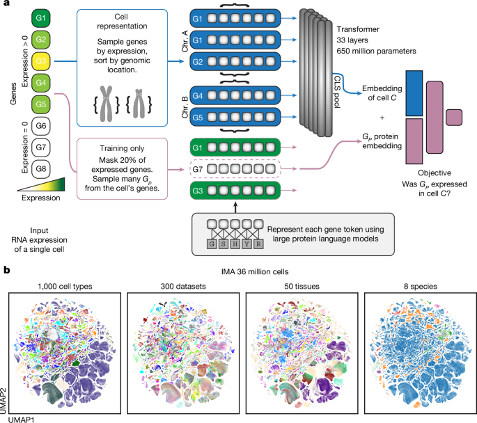
Overview of UCE

UCE is a machine learning model for mapping single-cell gene expression profiles into a universal embedding space, denoted as \(\mathcalU\). In this space, each cell c_i is represented as a d_emb-dimensional vector, where d_emb = 1,280. For all analyses we use the 1,280 dimensional UCE representation and not a two-dimensional embedding such as that generated from t-distributed stochastic neighbour embedding or UMAP. Users of UCE should rely on the full 1,280-dimensional representations to judge distances between cells, rather than data visualization using these methods, especially when they expect to see strong biological differences.

The model takes as input a dataset \(\mathcalD\) with N cells \({\\bfc_i\}_i=1^N\). Cells in \(\mathcalD\) can be drawn from one or more distinct scRNA-seq experiments. Each cell c_i in \(\mathcalD\) is described by a gene expression vector \(\bfx^i\in \mathbbN^K_i\), where K_i is the number of genes measured in c_i and can differ across \(\mathcalD\). The gene expression vectors \(\bfx^i\in \mathbbN^K_i\) are not subset to those with high variance. UCE defines a function \(f_u:{\{\rm\mathbbN^K_i\to {\rm\mathbbR}^d_\mathrmemb\}}_i=1^N\) that maps each gene expression vector xⁱ to its cell embedding vector hⁱ.

Model input: gene representation

The expression of gene g in cell c_i is denoted by \(x_g^i\), where g represents any protein-coding gene. The corresponding token embedding p_g is a pretrained embedding for the protein(s) encoded by the gene g. These embeddings are derived from a pretrained protein language model that takes an amino acid sequence as input and returns a d_p-dimensional embedding vector as output. To create P_g, we take the average of all proteins coded by gene g. In the context of UCE, we can formulate this as a dictionary that maps each gene g to a d_p-dimensional protein embedding vector. Specifically, we used the ESM2 model, which yields embeddings of size d_p = 5,120 (refs. ^32,33).

Protein language models are chosen for gene representation because they can generate universal representations of any protein sequence. Thus, for new species, all that is required is to have the amino acid sequences of that species’ protein coding genes. These genes do not need to have solved structures and orthology does not need to be calculated between them and the existing training data. Model training ablations demonstrate that, among a class of different protein language models, UCE models trained with ESM2-15B performed the best (Supplementary Fig. 8). Model ablation experiments further demonstrate that the use of protein embeddings to tokenize genes has substantial benefits for the more poorly represented species in the training corpus, as a small ablation model trained with protein embeddings outperformed a model with randomly initialized embeddings on all species except for human (Supplementary Fig. 8). Moreover, the use of protein embeddings enables a unique capability: embedding new species not found in the training data (Fig. 2).

Model input: cell representation

For each cell c_i in the input dataset \(\mathcalD\), we identify two distinct sets of protein-coding genes: the expressed genes \(G_i^+\) and the non-expressed genes \(G_i^-\). These sets are defined as follows:

For producing the cell embedding, a multi-set of 1,024 non-unique genes \(G_i^s\) are sampled from the expressed genes \(G_i^+\), with replacement. The probability of sampling a gene \(g\in G_i^+\) is weighted by the log-normalized expression of that gene, which can be formulated as:

where \(x_g^i\) is the expression count of gene g in cell c_i, and the sum in the denominator is over all genes in \(G_i^+\).

Note that, for a given cell, different random seeds can yield different sampled gene subsets and therefore slightly different representations (Supplementary Table 11); however, using a fixed seed selects the same genes each time and produces an identical embedding for repeated runs on the same cell.

Once the multi-set \(G_i^s\) is compiled for each cell c_i, we arrange the genes within each chromosome according to their genomic positions. Different chromosomes are specified using special chromosome start and end tokens. Start tokens are unique to each chromosome and species. Every chromosome group is combined into a single sequence, with chromosome order randomly determined. A cell-level CLS token is appended to the start of the sequence. It is designed to capture the cell-level embedding after training the model. The final sequence of genes ordered by genomic location and separated by chromosome is referred to as the cell sentence S_i for cell c_i.

Ordering the genes using this information does appear to have a positive effect on model performance (Supplementary Note 4 and Supplementary Table 3). Transformer models do not require any ordering of their inputs, and these metadata were added to the model only to enable potential applications, such as examining chromosomal aberrations or synteny between species. Future models of this type may choose to exclude this metadata, or include it using other methods besides positional encodings.

Transformer architecture

Each cell sentence S_i is fed into a transformer that consists of n_lay layers. Each layer contains a multi-head self-attention mechanism with n_head attention heads and a feedforward network operating over a hidden space of dimensionality d_hid. We also initialize sinusoidally-varying positional embeddings. Gene token embeddings are compressed using a single layer MLP to d_emb-dimensional vectors before passing through the transformer.

While the transformer architecture is highly performative, it requires substantial computational cost to train and evaluate. One important aspect of this cost is the quadratic increase in the runtime of transformers’ attention operations proportional to the number of tokens. Such a relationship requires that the number of genes sampled by UCE, 1,024, be relatively limited, especially given that individual cells might have more than 1,024 uniquely expressed genes. Future model architectures could explore increasing this context length, or using models with subquadratic scaling such as state space models⁵⁷.

Model output: cell embedding

The final output from the model is the cell embedding vector \(\bfh_\mathrmcell^i\in \mathcalU\), which corresponds to the d_emb-dimensional embedding of the CLS token in the final layer of the model following decoding with an additional MLP.

When cells with unrealistic random gene expression patterns, such as those generated by shuffling the expression of real cells, are inputted, the resulting cell embeddings default to a heterogeneous, out of distribution output (Supplementary Fig. 1).

Model training: cell representation

At the time of training, we generate a set \(G_i^M+\subset G_i^+\) by randomly selecting a certain percentage (r_mask) of genes from \(G_i^+\), without replacement. This set is used for computing the loss during training, and is masked from the cell representation.

The probability of sampling a gene \(g\in G_i^+\backslash G_i^M+\) (equation 3) is then updated to be:

We also establish two additional gene sets to be used for loss computation: \(G_i^L+\in G\) and \(G_i^L-\in G\). \(G_i^L+\) and \(G_i^L-\) are randomly selected from the masked set of expressed genes \(G_i^M+\) and the set of unexpressed genes \(G_i^-\), respectively. Both \(G_i^L+\) and \(G_i^L-\) are of equal size, specifically N_loss/2. In the case of \(G_i^L-\), the sampling is done without replacement unless \(| G_i^-| < N_\mathrmloss/2\). Similarly \(G_i^L+\), is also sampled without replacement unless \(| G_i^M+| < N_\mathrmloss/2\). In this case, \(G_i^M+\) is used as is along with additional samples drawn with replacement from the full set of expressed genes \(G_i^+\).

Model training: loss function

UCE is trained to reconstruct the binarized expression of genes in a cell, when those genes are masked from the model by setting their expression to 0. To calculate the loss function for a given cell c_i, the cell embedding vector \(\bfh_\mathrmemb^i\) is individually concatenated with every gene g within both \(G_i^L+\) and \(G_i^L-\). These concatenated vectors then serve as input to a feedforward multilayer perceptron (MLP), which computes the probability that gene g is expressed within cell c_i.

\(\bfh_\mathrmcell^i\) represents the embedding vector for cell c_i and p_g represents the token embedding for gene g. Then the concatenated vector \(\bfz_g^i\) that serves as input to the MLP for cell c_i and gene g is:

where ∣∣ denotes the concatenation operation and \(\bfp_g^\prime \) is the compressed protein embedding.

The MLP then processes this concatenated input to produce the predicted probability that gene g is expressed:

This probability is then used in the binary cross-entropy loss function. The true classification labels for each gene’s expression status in cell c_i are represented by the vector yⁱ. UCE is trained to accurately predict the expression of genes in \(G_i^L+\) and the lack of expression in \(G_i^L-\). The model is trained using a binary cross-entropy loss, which is averaged across all N_loss genes and all N cells in the minibatch as follows:

Further details on hyperparameter choices are provided in Supplementary Table 2. Different hyperparameter choices for this masked loss can impact final model quality. Reducing the masking percentage from 20% to 10% or increasing it to 40% did not improve model performance (Supplementary Note 4 and Supplementary Table 4). In future models, an alternate loss, for example, a generative decoder style loss, could be used, and might improve performance as no genes would be masked during training.

Creating IMA and dataset preprocessing

The IMA that was used to train UCE was created by combining scRNA-seq datasets from multiple publicly available sources. The majority of IMA data (33.9 million cells and 285 datasets) are human and mouse data downloaded from CZI Cell X Gene (CxG) Census³⁵ v.2023-07-10 (10 July 2023). Duplicate cells were removed by selecting primary cells only. The remainder of the IMA is composed of 2.3 million cells from 28 datasets, from eight different species: human, mouse, zebrafish, rhesus macaque, crab-eating macaque, mouse lemur, frog and pig.

For datasets from the CxG Census, preprocessing involved only filtering cells by minimum gene counts (200) and genes by a minimum cell counts of 10. No highly variable gene selection was applied. For datasets collected from other sources, preprocessing was not uniform (Supplementary Note 1).

For visualization of the IMA (Fig. 1b), predicting green monkey cell types (Fig. 2d), matching new species centroids (Supplementary Table 15) and prediction of Norn-like cells (Fig. 4 and Extended Data Fig. 9), a representative sample of the IMA was used in place of the full 36 million cells. This representative sample was used to speed up computationally intensive tasks like UMAP calculation. The sample was created by randomly choosing 10,000 cells from each dataset, without replacement. For datasets with fewer than 10,000 cells, the entire dataset was included. In total, this representative sample has 2,969,114 cells. The average number of cells per dataset in the sample is 9486. For visualization and centroid calculation, cell types in the sample were coarsened by mapping them to a set of 51 coarse cell types (Supplementary Table 19).

Model Evaluation

• Zero-shot embedding quality and clustering: for evaluating the quality of embeddings, we used metrics from the single-cell integration benchmark¹⁶.

• Cell type organization: for each cell type dendrogram the Euclidean distance was used to perform hierarchical clustering across all cells.

• Comparison to cell ontology: here, we used the tree distance between any two cell types in Cell Ontology⁴⁸. We used the Cell Ontology from release date 16 August 2016. To determine the Euclidean distance distribution, we sampled 100,000 random pairs of cells from Tabula Sapiens v.2.

• Zero-shot cell type alignment to IMA: for each cell type θ, a centroid was identified separately for data from Tabula Sapiens v.2 (TSv2) \(c_\theta ^T\) and from IMA \(c_\theta ^I\). For each cell type that is present in both TSv2 and the IMA, the three nearest-neighbour cell type centroids \(\bfN_\theta ^T\) to the centroid in Tabula Sapiens \(c_\theta ^T\) were identified. These neighbours could be either from Tabula Sapiens or from the IMA. If this set of neighbours \(\bfN_\theta ^T\) to the anchor centroid from TSv2 data \(c_\theta ^T\) contains the centroid for the same cell type in IMA data \(c_\theta ^I\), then this was counted as a correct match. This analysis was performed per tissue, both in the UCE embedding space as well as in the original expression space (after log-normalization). In the case of the original data representation, the set of 5,704 shared genes across all 184 human datasets in the IMA was used to represent each cell. The expression counts in each cell are normalized by total counts over all genes, so that every cell has the same total count after normalization. This is followed by a log transformation. This follows standard Scanpy data preprocessing guidelines⁵⁸.

• Scanpy analyses and package versions: unless otherwise stated, all analyses were performed using Python v.3.7+ and scanpy v.1.9.3+. The default settings were always used unless otherwise specified. For differential expression analyses, the scanpy function sc.pp.highly_variable_genes was used with the default settings with the flavour seurat_v3. Scanpy was also used to generate all UMAPs. First, sc.pp.neighbours was run, using the default settings except for setting use_rep to the correct embedding value, such as the embedding from UCE. Then sc.tl.umap was used with the default settings to generate the UMAP. The evaluation framework for UCE is released with the following versions: numpy v.1.26.4, scipy v.1.14.1, pandas v.2.2.2, tqdm v.4.66.5, torch v.2.1.1, scanpy v.1.10.2, accelerate v.0.24.0, and for downloading model files: requests v.2.25.1, urllib3 v.1.26.6.

Description of other models

• Geneformer²⁷ is a transformer-based foundation model. Geneformer represents a cell as a list of genes sorted by their expression. Geneformer was trained using masked language modelling on 30 million cells. For all analyses, the GF-12L-30M-i2048 model was used.

• tGPT⁵⁹ is a transformer-based foundation model. tGPT represents cells, like Geneformer, as a list of genes sorted by expression. However, tGPT is trained as an autoregressive language model, rather than a masked language model. tGPT was trained on 22.3 million cells.

• scGPT²⁸ is a transformer-based foundation model. scGPT represents cells as a list of the expression values of its genes. scGPT is trained to iteratively decode those genes’ expressions when some are masked, using generative pretraining. scGPT was trained on 33 million cells. For all analyses, the whole-human model was used.

• scVI¹⁵ is a variational autoencoder. scVI is trained to reconstruct gene expression values using a zero-inflated negative binomial loss. scVI was used with the default parameters for all experiments. scVI v.1.01+ was used. scVI input datasets were transformed only by taking the highly variable gene subset using sc.pp.highly_variable_genes with the flavour seurat_v3, and then the scVI model was trained with the default settings (number of hidden variables, 10).

• scArches builds on the scVI architecture to enable transfer learning of cell types. As used in this work, scArches first trains an scVI model on a reference dataset, fine-tunes a cell-type-aware scANVI model using the cell types from the reference dataset and then further fine-tunes this model on a transfer dataset using architecture surgery. scArches was used with the default parameters for all experiments. scArches v.0.5.1 was used, and was trained using the same scVI model for the dataset as a starting point.

• For comparisons to PCA, the default scanpy settings and best practices were used. The dataset was normalized using sc.pp.normalize_total, which normalized cell counts to the median count value for the dataset. Expression values were then log normalized using sc.pp.log1p, and PCA was calculated with sc.pp.pca, which defaults to the top 50 principal components.

Norn cell differential expression

A logistic classifier was trained to predict cell types from UCE embeddings on mouse kidney cells. This classifier was then applied to UCE embeddings from the representative sample of IMA datasets. The datasets were then split by tissue, and the datasets with the most predicted Norn cells in each tissue were used for differential expression analysis. The top 13 kidney datasets, top 6 lung and top 6 heart datasets were chosen.

For each individual (full) dataset, RNA counts were log normalized, and then differential expression was run using default settings as implemented in Scanpy⁵⁸, comparing predicted Norn cells with all other cells in the dataset. The results of these differential expression tests were used to determine the log-transformed fold change of marker genes in predicted Norn cells (Fig. 4c and Extended Data Fig. 9).

Reporting summary

Further information on research design is available in the Nature Portfolio Reporting Summary linked to this article.