Regression to the mean can explain saturation of geomagnetic storms

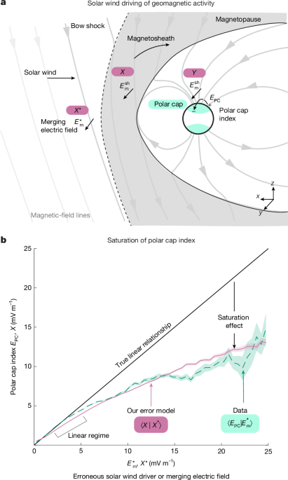
The most common symbols used are explained in the Extended Data Table 2.

Solar wind measurement uncertainty

There are several solar wind coupling functions that attempt to quantify the driving, one important one is the solar wind merging electric field or merging geoeffective field \(E_\rmm^* \) (refs. ^4,24).

This field is also known as the Kan–Lee electric field and is calculated from solar wind parameters at Lagrange point L1 alone²⁴. In equation 1.1, V_sw is the solar wind speed in km s⁻¹, \(B_\rmT,\mathrmsw=(B_y^2+B_z^2)^1/2\) is the transverse magnitude of the interplanetary magnetic field (IMF) in nT, and θ_sw = tan⁻¹(B_y/B_z) is the transverse IMF clock angle in radians. E_m is a positive-valued quantity with the units of the electric field (mV m⁻¹), reflecting the assumption that energy flows only from the solar wind to the magnetosphere. The above quantities are measured in geocentric solar magnetospheric (GSM) coordinates using spacecraft orbiting the L1 point approximately 230 R_E upstream from Earth. The GSM coordinates are convenient for studying the effects of the IMF components on magnetospheric and ionospheric phenomena. Its x axis points towards the Sun, and the z axis is the projection of Earth’s magnetic dipole axis onto the plane perpendicular to the x axis. For a purely southwards IMF, the merging electric field \(E_\rmm^* \) is equal to the solar wind electric field E_sw = V_x,swB_z, where V_x,sw is a component of the solar wind velocity along the x direction.

The dawn–dusk portion of the shocked solar wind convection electric field maps along the equipotential magnetic-field lines and drives the plasma convection down in the polar cap ionosphere. The convection corresponds to an electric field across the polar cap in the rest-frame of the Earth (E_PC). The PCI is a measure of this field and part of the energy input into the Earth’s magnetosphere. The index has gone through many iterations over the past 50 years, but it is essentially the maximum amplitude of variations observed from magnetometers near the South and North Poles^3,25,26. The current version of the index is scaled on a statistical basis of magnetic variations to the merging electric field, such that the index is highly correlated to the merging electric field. This makes the PCI independent of daily and seasonal variations and the local ionospheric properties. PCN is the index derived from the magnetometer in the northern polar cap and PCS is derived from the southern polar cap. We use the PCI as a proxy for E_PC (that is, PCI ≈ E_PC), as it combines both indices to provide a positive-valued index, which is more accurate than the individual indices²⁶. PCI = 0.5(PCS + PCN), with a condition that negative values of either PCS or PCN are set to 0. PCI or E_PC also has the units of the electric field, and several statistical analyses in the literature reveal that it is linearly proportional on average to the electric potential across the polar cap, called the cross-polar cap potential^11,27. Fluctuations in PCI can occur owing to nightside magnetosphere processes²⁸, but the above relation is still maintained on average.

The Kan–Lee electric field \(E_\rmm^* \) is only an approximation of the true driver of the magnetosphere, that is, the shocked solar wind plasma \(E_\rmm^\mathrmsh=V_\mathrmshB_\mathrmsh\sin ^2(\theta ^\prime /2)\), the value of which is not easily available to us (Supplementary Methods 2a). This leads to the uncertainty and nonlinear regression bias discussed in this work. Instead, we have only an erroneous estimate of the true coupling function approximately propagated to the polar cap, \(E_\rmm^* \). Hence, we need to reinterpret the literature as saying that low values of the erroneous estimate of the solar wind strengths \(E_\rmm^* \) (not \(E_\rmm^\mathrmsh\)) correlate linearly with the polar cap potential. And at high values of \(E_\rmm^* \), the polar cap potential saturates.

We calculate \(E_\rmm^* \) by using WIND satellite measurements published in the OMNIWeb database²⁹. The database provides the values corrected for the propagation delay of the solar wind from L1 to the bow-shock nose^30,31,32. Then as frequently done, we apply a further correction of a constant delay of about 17 min to account for the propagation delay from the nose to the polar cap ionosphere^16,33. Previous literature that discusses the polar cap potential saturation problem estimates \(E_\rmm^* \) similarly. We use the WIND data from 1995 to 2019 and the polar cap indices from the same time range. Both data are 1-min averages; larger time averages will lead to additional uncertainties³⁴. We only use data samples when both WIND measurements and polar cap indices are available.

\(E_\rmm^* \) can differ from the shocked solar wind driver in the magnetosheath \(E_\rmm^\mathrmsh\) in two ways. One is through a consistent deterministic bias that is determined by the bow-shock that slows down the plasma. This deterministic bias is nearly zero as the tangential (and the largest) component of the electric field across the bow-shock remains unchanged. We do not concern ourselves with this deterministic bias, as it will manifest in the data as a physical effect anyway. However, \(E_\rmm^* \) can also differ randomly from the true solar wind driver \(E_\rmm^\mathrmsh\), owing to fluctuations in the plasma properties caused by physical processes between L1 and the reconnection site, acting in random directions. These random fluctuations contribute to the uncertainty in \(E_\rmm^* \) when we use it as a proxy for the true driver \(E_\rmm^\mathrmsh\). This random error is concerning, as it does not average away, and manifests as a regression bias in data analysis and is easily confused as a physical effect, hence we calculate and correct for it.

We categorize the random uncertainty in \(E_\rmm^* \) relative to the true value \(E_\rmm^\mathrmsh\) into three primary sources.

1. (1)

   Uncertainty in propagation delay of the solar wind from L1 to the bow-shock nose (dt₁).

2. (2)

   Uncertainty in the propagation delay of the effect of solar wind forcing from bow-shock nose to the polar cap ionosphere (dt₂).

3. (3)

   Random variability in the shocked solar wind owing to spatial variation in the incoming solar wind and transformations of its plasma parameters during propagation through the bow-shock and the magnetosheath (ϵ).

Knowing the statistical distribution of the above uncertainty will allow us to construct a stochastic model of the estimate \(E_\rmm^* \) as a function of the true driver \(E_\rmm^\mathrmsh\) mapped to the polar cap ionosphere. In the following subsection, we develop a statistical error model of the estimate of the true shocked solar wind that drives the cross-polar cap convection from an estimate of its stochastic properties and uncertainty distributions. For the calculated uncertainties (Fig. 2c), the model predicts the polar cap potential saturation, which is strikingly similar to data from 25 years of observations (Figs. 1b and 2a,b).

Statistical error model

To distinguish between data and model, we replace \(E_\rmm^\mathrmsh\) with X when referring to the random variable corresponding to the shocked solar wind driver in the statistical model. We also replace the PCI, which is proportional to the convection electric field E_PC in the ionosphere, with a counterpart in the model Y_PC. Hence, in the model, X is the shocked solar wind driver accurately time-shifted to the polar cap, and X* is its erroneous estimate (that is, solar wind driver measured at L1 or \(E_\rmm^* \)). We hypothesize the following statistical error model:

We assume that X*, X, dt₁, dt₂ and ϵ are stochastic processes. In other words, they are each a collection of random variables in time (t ∈ T) with an associated probability distribution that determines the random value it might take at a given time t. Below we present our estimates of the probability distributions and autocorrelation functions of these stochastic processes. Using these estimates of X, dt₁, dt₂ and ϵ, we calculate X*. After which, we validate the model results by comparing them with the data \(E_\rmm^* \).

Input X

If reconnected open-field lines in the polar cap region do not have large parallel resistances, accurate mapping of the shocked solar wind electric field onto the polar cap should result in X, such that Y_PC ∝ X. In agreement with this, in data, we see that the probability density function (PDF) of the PCI index or E_PC (and hence Y_PC) and solar wind driver \(E_\rmm^* \) are very similar, implying that the distribution of Y_PC is also similar to X. As a result, we assume that the PDF of X is similar to the PDF of E_PC (and \(E_\rmm^* \)) that we can estimate from data. It is noted that this is not surprising as E_PC is constructed to be highly correlated with \(E_\rmm^* \), and from Kan and Lee’s arguments \(E_\rmm^* \) is also correlated with \(E_\rmm^\mathrmsh\), and hence all these parameters have similar PDFs. (Although we have measurements of \(E_\rmm^\mathrmsh\) from near-Earth orbiting spacecraft, they are discontinuous and hence do not directly provide an unbiased PDF of X). Like many solar wind parameters, E_PC and \(E_\rmm^* \) can be approximated to be a log-normal distribution²⁰. Therefore, we assume the PDF of model input X to be a log-normal distribution that closely fits the PDF of E_PC from data (Extended Data Fig. 2a). We also assume that the adjacent values of X in time are correlated similarly to adjacent values of E_PC in time (Extended Data Fig. 2b), as fluctuations in time of shocked solar wind electric field should correlate with that of the cross-polar cap electric field in the ionosphere. In other words, we assume that in our model, X shares the stochastic properties of the PCI or electric field E_PC. If the assumption fails, the results of the model, particularly the second-order statistics, will be inconsistent with what is observed in the data. Finally, we assume that X is a stationary process, that is, its probability distribution and autocorrelation function does not change with time.

Uncertainty in propagation delay from L1 to nose dt
₁

Solar wind parameters measured upstream are time-shifted to account for the delay in propagation of the wind to the bow-shock nose. Case and Wild estimate the uncertainty to be on the order of minutes³⁵. On the basis of their results and consistent with other studies³⁶, we assume dt₁ to be an independent random process with a PDF of a Student’s t-distribution with shape factor 1.3, mean 0, and scale parameter approximately 8 min (Extended Data Fig. 2c and Supplementary Methods 2b). The distribution is zero mean and has a longer tail than the normal distribution.

Uncertainty in propagation delay from nose to polar cap dt
₂

Changes in the dayside shocked solar wind electric field propagate along equipotential open magnetic-field lines to the polar caps. The delay in this propagation is on average about 17 min¹⁶ but can vary from −5 min to 50 min²⁷. Historically, researchers have used a constant propagation delay (t₂) of about 10–30 min^37,38 for this stage of propagation. However, the uncertainty of propagation time here is significant. We model the PDF of t₂ as a Weibull distribution with mean approximately 17 min¹⁶, standard deviation approximately 25 min and shape factor 1.3 (Extended Data Fig. 2c and Supplementary Methods 2b). The Weibull distribution keeps the total delay t₂ + dt₂ positive and captures the broad spread in the propagation delay^16,26,27.

Magnitude uncertainty ϵ

There are several other reasons for the magnitude of the shocked solar wind driver to be randomly different from its proxy measured at the L1. The IMF clock angle could change substantially after crossing the bow-shock, spatial variations in the solar wind can lead to a different part of the wind interacting with the Earth’s magnetosphere, and changes in the magnetospheric state or its history can lead to changes in the local plasma and field conditions in the magnetosheath. As the solar wind strength increases, the random variation in the field can increase owing to the increased spatial structuring of the solar wind, and any clock-angle variation during increased field strength can lead to larger variations in geoeffectiveness.

To estimate these random variations, we use direct evidence from a database of simultaneous measurements of plasma and field strengths in the magnetosheath. Using a gradient boost classification algorithm, measurements from near-Earth satellites such as THEMIS, MMS, DoubleStar and Cluster, are classified into solar wind, magnetosheath and magnetosphere regions³⁹. Our interest is in the measurements made within the magnetosheath, close to the magnetopause in the subsolar region (|Y| < 5 R_E and |Z| < 5 R_E). The distance from the magnetopause boundary is determined using a machine-learning-based empirical model of the boundary, which performs better than other magnetopause models available in the literature⁴⁰. For specific values of the magnetosheath measurements (\(E_\rmm^\mathrmsh\)), we calculate the variance in the measurements made at L1 and time-shifted to the bow-shock (\(E_\rmm^* \)). This variance is an estimate of the uncertainty in the solar wind driver \(E_\rmm^* \) for a given value of the shocked solar wind driver \(E_\rmm^\mathrmsh\). The ‘magnitude uncertainty’ ϵ is set to the same variance, and we model it as a zero-mean Gaussian with a standard deviation that varies with the magnitude of X according to data. The magnitude uncertainty is not constant with the strength of the shocked solar wind driver, instead it increases until \(E_\rmm^\mathrmsh\approx 12\,\mathrmmV\,\rmm^-1\), after which the statistics become poor and an accurate estimate of the variance becomes challenging (Supplementary Methods 2b). In this regime, we estimate the uncertainty in the solar wind driver relative to measurements of near-Earth satellites just upstream of the bow-shock (approximately 10 < X < 50 R_E). This uncertainty will be the minimum uncertainty for values >12 mV m⁻¹ (that is, a conservative estimate of the uncertainty), and this remains roughly the same with increasing shocked solar wind driver value. Figure 2c shows the relative error, σ(ϵ)/X, and how that varies with X. The heteroskedastic behaviour of this uncertainty is consistent with the observed statistical variations in the difference between solar wind driver and the PCI shown in Extended Data Fig. 3d,e. The variation in their difference increases up to a PCI of approximately 12 mV m⁻¹ and then remains constant. We also assume that ϵ has an autocorrelation function similar to that of the difference between the observed solar wind driver \(E_\rmm^* \) and the polar cap index PCI ≈ E_PC.

Using the above estimates of uncertainties, we generate an ensemble of time series of X, dt₁, dt₂ and ϵ, and calculate the corresponding time series of the erroneous estimate X* using equation (1.2). The statistical properties of the model output agree remarkably with that of the data.

Validation of error model

We validate this nonlinear error model by comparing the second-order statistics of the error model parameters with that of their counterparts in data. The error model predicts the PDF of the solar wind driver \(E_\rmm^* \), the standard deviation of the normalized error, the conditional normalized error distribution and finally the regression bias stemming from the regression to the mean effect. This validation is the rationale for using the error model and is presented in the Supplementary Methods 2b. Here we also discuss a sensitivity analysis of the nonlinear regression bias, which increases with increasing uncertainty in the time of propagation, and with increasing uncertainty in the magnitude uncertainty ϵ (Extended Data Fig. 4). The analysis shows that output of the error model is robust to the input uncertainties and variance of input X. Supplementary Methods 2d summarizes the full computer code used.

Correcting the error

The regression bias b = X* − ⟨X|X*⟩, which is the consistent deviation between the measurement and the likely true value given the measurement. The erroneous measurement X* can now be corrected to X^c by subtracting the bias from it X^c = X* − b, which simply reduces to X^c = ⟨X|X*⟩. Crucially, from the model output, we can calculate the conditional expectation of the true value given the erroneous estimate: f_r(x) = ⟨X|X* = x⟩, that is, we have a statistical, functional relationship between the true value and the erroneous measurement. For the particular assumptions of uncertainties in measurement, f_r(x) is the best estimate of the true value (X^c or \(E_\rmm^\rmc\)) given the erroneous value (X* or \(E_\rmm^* \)). Therefore, f_r(x) can be used to statistically correct the erroneous estimate \(E_\rmm^* \) to a most likely estimate of the true value \(E_\rmm^\rmc\). \(E_\rmm^\rmc\) is useful for revealing the true statistical correlation with other variables, such as the PCI (E_PC) or auroral current strengths (SML). The process of statistically correcting for the uncertainty using the conditional expectation of the true value given the erroneous estimate \(E_\rmm^\rmc=f_\rmr(E_\rmm^* )\) for an unbiased regression analysis is called regression calibration¹⁹. Figure 3 shows the results of this calibration. SML is the westward auroral electrojet index from the SuperMAG database, which is a measure of the westwards currents flowing in the auroral regions^41,42. It is calculated using ground magnetometers and procedures completely independent of the calculation of the PCI. As regression calibration of \(E_\rmm^* \) to \(E_\rmm^\rmc\) results in a linear relationship between both \(E_\rmm^\rmc\) and E_PC (Fig. 3a) and \(E_\rmm^\rmc\) and SML (Fig. 3b), it suggests that our findings are independent of the construction of the ionospheric response variables. The confidence intervals shown in Figs. 1–3 provide only an estimate of the reliability of the regression procedure, that is, it means 95% probability that repeating the procedure will contain the regression curve and does not imply that the true value or the true regression curve will lie within the confidence interval with a 95% probability.

Temporal uncertainty can lead to a nonlinear regression function

In Supplementary Methods 2c, we analytically derive the following general result that temporal uncertainty in measurement can lead to a perception of nonlinearity in a linear system’s correlation response. For a linear system with response Y, input X, and the input with measurement error W = X(t + Δ), the biased system response ⟨Y|W⟩ is a function \(f_\rmr^* (w,\sigma _\delta /k)\). Here σ_δ is a measure of the random uncertainty Δ in the time of measurement and k is the autocorrelation time constant. The system response is a function of the ratio σ_δ/k. This ratio is a measure of uncertainty in the time of measurement. We numerically integrate the function, which is fully described in equation (1.21) in Supplementary Methods 2c, within the ranges of Δ for specific values of σ_δ/k and generate Extended Data Fig. 4c. The figure shows that \(f_\rmr^* (w,\sigma _\delta /k)\) varies nonlinearly with w when there is temporal uncertainty.