


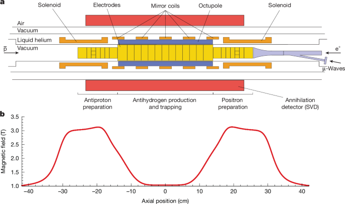
Trap magnetic field profile, stabilization and characterization
The design of the flattened magnetic field profile along the axis at the centre of the trap in the trapping region, shown in Fig. 1, represents an important component of the gains in frequency resolution reported here. In particular, the curvature of the magnetic field governs the timescale over which anti-atoms interact with the microwave field as they are brought into resonance. In round numbers, the second axial derivative of the axial magnetic field profile used in the current work is less than 2 T m−2, or a factor of 20 smaller than that of the (unflattened) trapping field used during the measurement of the hyperfine splitting reported in ref. 15. This, in turn, enhances positron spin-flip efficiencies and our ability to probe anti-atoms much closer to the minimum frequencies of the two transitions. However, unlike the maximally flattened field configurations used in previous optical spectroscopy experiments13,39, here we intentionally depress the field below the central mirror coil by about 5 × 10⁻⁵ T to ensure the existence of a shallow, centrally located absolute minimum (Extended Data Fig. 1).
We use the electron cyclotron resonance (ECR) technique to map the axial magnetic field profile along the axis of the trap in situ with a frequency resolution of the order of 1 ppm (ref. 32) and a spatial resolution of about 1 mm, and are thus able to directly confirm the formation, location and depth of the central magnetic field minimum along the axis. Moreover, we use ECR to independently resolve and characterize both the initial field drift (attributed to fine-scale flux relaxation or redistribution after the first ramp up of the superconducting magnets at the beginning of the experiment) and the subsequent long-term downward linear field drift (attributed to the decay of persistent currents in the external solenoid used to generate the 1 T background field). These studies show that the drifts depend on the time history of magnet operations. Consequently, magnets are energized in the same sequence in all experiments.
For each experiment, we perform ECR measurements after the magnetic trap is energized as well as after each replicate as a complementary monitor of the magnetic field drift. From a linear fit to the ECR magnetic field measurements following each replicate, we extract a linear magnetic field drift of −0.025 ± 0.001 G h−1 for the 1.03 T experiment and −0.026 ± 0.001 G h−1 for the 1.07 T experiment (Extended Data Fig. 2). Assuming the same magnetic field dependence as in hydrogen, this corresponds to expected positron spin resonance onset frequency drifts of −71 ± 3 kHz h−1 for the 1.03 T experiment and −73 ± 3 kHz h−1 for the 1.07 T experiment. This is consistent with the measured linear drift of the positron spin resonance frequencies of −72.82 ± 0.04 kHz h−1 for the 1.03 T experiment and −75.64 ± 0.05 kHz h−1 for the 1.07 T experiment we find in our analysis (Fig. 4). Note that ECR measurements of the on-axis magnetic field were used solely to characterize magnetic fields in preparation for the experiments described here and as a complementary magnetic field measurement. ECR measurements were not used in our extraction of the ground-state hyperfine splitting of antihydrogen.
During our experiments, the mirror coils are supplied with currents ranging from a few amperes to nearly 500 A. The octupole is operated with a current of 900 A. These currents are individually monitored using high-precision, ultrastable direct current–current transformers based on closed-loop fluxgate magnetometer sensors (ITZ 2000-SB FLEX ULTRASTAB from LEM International SA). The DCCT provides a ±10 V output with a 500 kHz small-signal bandwidth. This signal was digitized by 24-bit National Instruments NI-9239 cRIO (Compact Real-time Input Output) analog-to-digital converter modules at 50 kS s−1 and averaged by the cRIO FPGA (field programmable gate array) firmware to 10 kS s−1. The resulting averaged signal was used for proportional–integral–derivative (PID)-based closed-loop control of the magnet power supplies, stabilizing output currents to within several mA.
Extracting the zero-field ground-state hyperfine splitting
The Breit–Rabi formula40 gives the following energy levels of hydrogen (Fig. 2a) in a magnetic field:
$$E_d=\fraca_1\rmS4+\frac12g_\rme\mu _\rmBB\left(1-\fracg_\rmpm_\rmeg_\rmem_\rmp\right),$$
$$E_c=-\fraca_1\rmS4+\frac12{\left[a_1\rmS^2+\left(g_\rme\mu _\rmBB\left(1+\fracg_\rmpm_\rmeg_\rmem_\rmp\right)\right)^2\right]}^1/2,$$
$$E_b=\fraca_1\rmS4-\frac12g_\rme\mu _\rmBB\left(1-\fracg_\rmpm_\rmeg_\rmem_\rmp\right),$$
$$E_a=-\fraca_1\rmS4-\frac12{\left[a_1\rmS^2+\left(g_\rme\mu _\rmBB\left(1+\fracg_\rmpm_\rmeg_\rmem_\rmp\right)\right)^2\right]}^1/2,$$
where μB is the Bohr magneton, ge and gp are the electron and proton g-factors, and me and mp are the electron and proton masses. By taking the difference of the transition frequencies, the magnetic field terms of the Breit–Rabi formula cancel and the hyperfine splitting a1S/h is extracted. Here, we assume that the ground-state energy levels of antihydrogen follow the same functional form as in hydrogen, and thus a1S/h = fda(B) − fcb(B) for any B, but the zero-field hyperfine splitting and magnetic field scaling coefficients may differ.
Microwave magnetic field and positron spin-flip rates
Microwaves are produced using an Agilent E8257D PSG analog signal generator, amplified using a Miteq AMF-4B amplifier, and simultaneously matched to the ALPHA-2 apparatus in the vicinity of frequencies needed for spectroscopy using an E–H tuner. They enter the ultrahigh vacuum region of the apparatus through a custom-built vacuum window and propagate down a waveguide to the electrode stack, in which they enter the trapping volume, as shown in Fig. 1. A characterization of the microwave hardware was conducted using a Keysight model N5224B PNA Microwave Network Analyser. The signal generator output frequency is referenced to a 10 MHz signal provided by CERN, which has a precision better than 10−6 Hz. The signal generator calibration was verified before spectroscopy experiments were performed.
The positron spin-flip transitions are driven by the component of the microwave magnetic field that is transverse to the static axial magnetic field at the centre of the trap. Therefore, we are interested in balancing the amplitudes of this component of the microwave magnetic fields at frequencies in the vicinity of the |c⟩ → |b⟩ and |d⟩ → |a⟩ onset transition frequencies. We do this with ancillary microwave power studies, in which the lineshapes are compared for different injected powers using large samples of antihydrogen atoms (roughly 5,000). Injected powers (Extended Data Table 1) were chosen such that |c⟩ → |b⟩ and |d⟩ → |a⟩ lineshapes match as closely as possible. Differences in injected powers between phases 1 and 3 are the consequence of the strong frequency dependence of the power that reaches the anti-atoms. Any remaining imbalance of the positron spin-flip rates contributes to the overall systematic uncertainty (signal model in Table 1 and Methods, ‘Systematic uncertainties’). During phases 2 and 4, the injected powers were increased to more quickly remove the remaining |c⟩– and |d⟩-state atoms, respectively. In both experiments, the number of annihilations attributed to |c⟩-state atoms was consistent with the number attributed to |d⟩-state atoms (Extended Data Table 1). This is consistent with the assumption that the two states are produced in equal amounts during formation and removed from the trap at consistent rates during the microwave sweeps.
Data acquisition and selection
Antihydrogen annihilation events are reconstructed from their charged-particle products, which are detected by the SVD as described in previous experiments13,41. Annihilations are separated from the cosmic-ray background using machine-learning procedures based on a Boosted Decision Tree classifier42. The efficiency for annihilation event candidate selection is 75.7%, and the rate at which cosmic rays are misidentified as signal is 37.4 × 10⁻³ s−1.
Higher rates of background events as compared with the expected cosmic-ray contribution may result from factors ranging from antihydrogen annihilation on residual gas to microwave ejection of remnant trapped |c⟩-state anti-atoms in Phase 3 as they come into resonance at higher magnetic fields. In our analysis, we make no attempt to disentangle different sources of background.
Annihilation events occurring during the frequency settling time (8–30 ms) between each microwave irradiation step are removed from the dataset. The remaining events are binned according to the frequency of the microwave radiation injected in the trap at the time of the annihilation.
Data analysis
The distributions for each transition from each replicate of our experiment are fitted with an empirical model, defined by the convolution of a base lineshape function, g, and a resolution function, R, on top of a constant background, whose normalizations are free parameters of the fit. The base lineshape function is zero for frequencies below a given threshold, which we refer to as the onset frequency (fo), and monotonically rises as the resonant volume increases and decays as the antihydrogen population is depleted. The resolution function accounts for broadening effects that smooth the lineshape, such as Doppler broadening, transit-time broadening and fluctuations in the magnetic field.
The g function assumes the following form:
$$g(\barx)\propto \left\{\beginarraycc0 & \barx < -\sigma (k+1),\\ \exp \left(-\frac12\right)\times \left[\frac\barx+\sigma (k+1)\sigma k\right]^k & [\barx\ge -\sigma (k+1)]\vee (\barx < \sigma ),\\ \exp \left(-\frac\barx^22\sigma ^2\right) & (\barx\ge -\sigma )\vee (\barx < 0),\\ \exp \left(-\frac\barx^22\sigma _\rmr^2\right) & (\barx\ge 0)\vee (\barx < \sigma _\rmr),\\ \exp \left(-\frac12\right)\times \left[\frac\barx+\sigma _\rmr(n-1)\sigma _\rmrn\right]^-n & \barx\ge \sigma _\rmr.\endarray\right.$$
Here, \(\barx=x-[\,f^\rmo+\sigma (k+1)]\) and fo is the frequency threshold below which the piecewise function g is zero and above which it features a power-law rise, corresponding to the rapid increase in resonant volume. The core of g consists of an asymmetric Gaussian, followed by a power-law tail, which describes the region in which the annihilation counts decay due to the declining antihydrogen population for the state under study. The widths σ and σr of the asymmetric Gaussian core control the rise and decay lengths, respectively. The parameters k and n govern the power-law rise and decay, respectively.
Frequency sweeps proceed monotonically upwards, so our resolution function is asymmetric and defined as
$$R(\barx)\propto \left\{\beginarraycc\exp \left(-\frac\barx^22\sigma _\rmb^2\right) & \barx\ge 0,\\ \exp \left(-\left|\fracx\xi _\rmR\right|\right) & \barx < 0,\endarray\right.$$
where \(\sigma _\rmb\) is the broadening parameter and the right-sided exponential decay with a negligible width \(\xi _\rmR=0.2\,\mathrmkHz\) is included to ensure continuity.
For each magnetic field dataset, we perform one combined fit across all eight replicates for the |c⟩ → |b⟩ transition (Phase 1 annihilations) and another combined fit across the eight replicates for the |d⟩ → |a⟩ transitions (Phase 3 annihilations). The fit parameters controlling the lengths of the rising and falling edges of the empirical base function (n, σ, σr) are shared between all replicates but are allowed to differ between |c⟩ → |b⟩ and |d⟩ → |a⟩ transitions to accommodate residual differences in the respective spin-flip rates. For example, Fig. 3 shows a slightly larger lineshape width for the |d⟩ → |a⟩ transition compared with the |c⟩ → |b⟩ in the 1.03 T experiment. This indicates that the spin-flip rates at the |d⟩ → |a⟩ frequencies are slightly lower than at the |c⟩ → |b⟩ frequencies, despite our attempts to balance them in preparatory measurements (as described above). The parameters describing the steepness of the rising edges and the width of the resolution functions are fixed according to fits to simulated data (see below) of the experiment to be k = 2 and σb = 10 kHz, respectively, for both transitions. The uncertainties associated with these choices are discussed below. Only the onset frequencies, \(f_\textcb^\rmo\) and \(f_\textda^\rmo\), as well as the normalizations for the signal and background are allowed to vary for each repetition. The combined fits for each magnetic field dataset, therefore, yield eight pairs of onset frequency markers.
The magnetic field conditions for each of the replicates are different because the two transitions are probed at different times (separated by 812 s) while the magnetic field is drifting. To account for this effect, the two sets of onset frequencies are fit with a model function comprising two straight lines with a common slope whose separation in frequency is our estimate of a1S/h, as shown in Fig. 4. The other fit parameter is the average of the two intercepts.
The distributions of the two histograms for a specific replicate are shown in Fig. 3. For each experiment (1.03 T and 1.07 T), a simultaneous maximum likelihood fit is performed to the eight replicates.
Simulations
To inform two parameters of our model and study the associated systematic uncertainties we use simulations of the antihydrogen motion in the trap and the interaction with microwaves, reflecting the experimental frequency ramp and a magnetic field model tuned according to ECR measurements. Although these simulations cannot fully model the observed lineshapes at the required precision for this experiment because of the lack of knowledge of the microwave field and the static magnetic field off-axis, they offer a method to study the sensitivity of the lineshapes to different microwave powers and magnetic field profiles.
Simulations of antihydrogen motion in the ALPHA-2 trap were similar to those described in ref. 43. Positron spin resonance transitions are driven by the oscillating magnetic field component of the microwave field. Because we do not have knowledge of the position-dependent intensity of the microwave field, we use a position-independent intensity and polarization. To simulate positron spin resonance transitions, we performed a numerical, quantum two-state calculation in the resonance region. The detuning of each anti-atom was tracked in time and, when it was below 300 kHz, we calculated the quantum transition using the Crank–Nicolson algorithm with a time step of 39 ns. This quantum calculation uses the time-dependent magnetic field (hence a time-dependent detuning). After the atoms reach a detuning larger than 300 kHz, the probability of a transition is compared with a random number between 0 and 1. If the random number is less than the transition probability, then a spin flip was determined to have happened and the motion of the anti-atom is propagated using a flipped magnetic moment, pulling it towards the trap walls.
Systematic uncertainties
The following sources of systematic uncertainties were identified and estimated. The overall uncertainty budget is provided in Table 1.
Reproducibility
In the analysis, the annihilation distribution for each transition is assumed to be the same for the full duration of one experiment. However, the annihilation distributions may vary across the eight replicates. This could be due to the injected microwave frequencies reducing by roughly 900 kHz over the course of each experiment, because of the decaying solenoid magnetic field, which could change the microwave magnetic field strength seen by the anti-atoms and modify the annihilation lineshapes. These variations have, therefore, been considered as a source of systematic uncertainty. To estimate this contribution, we repeated the fit procedure with shape parameters of \(g(\barx)\) fixed using a fit to a high-statistics sample (consisting of roughly 5,000 anti-atom annihilations). These samples were collected following each experiment and had resonance frequencies of roughly 1,400 kHz and 1,200 kHz, respectively, lower than the first replicate of the 1.03 T and 1.07 T datasets. The difference in resonance frequencies between the midpoint of the eight replicates and the high-statistics sample was, therefore, similar to the frequency range spanned by the replicates (900 kHz). Because of this, we use the difference between our standard model and the one from the fit to the high statistics sample as a proxy for the typical variation that could be observed over the course of a measurement series.
To cross-check our estimated uncertainty, we repeated the nominal fit while removing the constraint that there is a common rise width (σ) for the eight replicates and let it vary for each. This yields values of the extracted hyperfine splitting that differ less than 2 kHz from the nominal results for both series, well within the estimated reproducibility term, with comparable statistical uncertainties.
Signal model
The |c⟩– and |d⟩-state antihydrogen atoms are obtained from the same synthesis process and are trapped in the same magnetic field profile; therefore, the lineshapes are expected to be subject to the same broadening mechanisms (motional broadening and Zeeman broadening). We also tune the injected power to match the two annihilation distributions. Barring effects associated with changing microwave powers over the frequency range of the experiment, addressed by the reproducibility systematic uncertainty, the same signal model should apply to both observed lineshapes. Because of this, and because our hyperfine splitting determination is a difference measurement, many potential systematic uncertainties associated with the signal model cancel out.
We evaluated the systematic uncertainty associated with the choice of base function by repeating the process using an alternative base model given by
$$g(\barx)\propto \left\{\beginarraycc0 & \barx < 0,\\ \left(\frac\barx\sigma \right)^k\times \exp \left\-\left(\frac\barx\sigma \right)^k+1\frac\sigma \sigma _\rmr\left(\frac1k+1\right)\right\ & (\barx\ge 0)\vee (\barx < \sigma ),\\ \exp \left\\frac\sigma \sigma _\rmr\left(\frackk+1\right)\right\\times \exp \left(-\frac\barx\sigma _\rmr\right) & (\barx\ge \sigma ).\endarray\right.$$
where σ and k are the length and sharpness of the rising edge and σr describes the exponential decay. The term \(\exp \left\\frac\sigma \sigma _\rmr\left(\frackk+1\right)\right\\) ensures continuity of the function at the maximum. This effect contributes 0.7 kHz to the systematic uncertainty of the hyperfine splitting at 1.03 T and 0.5 kHz at 1.07 T. We also varied the degree of the power-law rise, k, of the standard base function from 1 (a linear rise) to 5.4 (obtained by fits to high statistics data samples) to study the robustness of the result to the shape of the rising edge. This effect contributes 3.2 kHz and 4.2 kHz, respectively, to the systematic uncertainty at 1.03 T and 1.07 T.
We also evaluated the effect of our choice of resolution function with an alternative (one-sided cusp) model given by
$$R(\barx)\propto \left\{\beginarraycc\frac1\sigma _c\exp \left(-\frac\barx\sigma _c\right) & \barx < 0,\\ 0 & (\barx\ge 0).\endarray\right.$$
Based on this analysis, we conclude that our resolution functional form choice contributes 0.6 kHz to the systematic uncertainty of the measurement at 1.03 T and 0.3 kHz at 1.07 T.
Moreover, we estimated the effect of asymmetries in the two lineshapes by varying the σb parameters of the standard resolution function for the two transitions by ±2 kHz separately. This range is chosen based on fits to the simulated data over a range of microwave powers and represents a 20% difference (±2 kHz over 10 kHz) in the widths for the resolution functions between the two transitions. This effect contributes 3.5 kHz to the systematic uncertainty of the hyperfine splitting measurement at 1.03 T and 3.5 kHz at 1.07 T.
Finally, we studied the effect of varying the magnetic field profile (simultaneously for both transitions) in simulations. This resulted in a range of fitted σb values between 7 kHz and 13.6 kHz but had a negligible effect on the determined hyperfine splitting.
Binning
Binning is a source of systematic uncertainty, quantified as Δf/√6, because of the discrete nature of the scan and the fixed frequency separation between the Phase 1 and Phase 3 scans of each replicate. Uncertainties from the time of flight of the antihydrogen annihilation and synchronization have also been considered, by subtracting the 30 ms after each frequency transition from the event time and repeating the analysis. The difference with respect to the nominal case is found to be negligible.
B-drift
Deviations from the long-time (hours) linear decay assumption of the magnetic field have been explored with Gaussian Process Regression44 and considered in the uncertainty budget table. A limit to short-time (minutes) deviations from linearity, correlated with antihydrogen synthesis, has been obtained in auxiliary data by varying the interval between the synthesis and the spectroscopy phase of the experiment.
Validation and cross-checks
The signal-model-fitting algorithms were validated using Monte Carlo pseudo-experiments, in which synthetic experimental lineshapes were generated from the empirical model itself. The normalized residuals of the fitted parameters confirmed that the procedure was unbiased and that the associated uncertainties were accurately estimated.
To assess the sensitivity of the measurement to residual differences between the base lineshapes for the two transitions, the analysis in Fig. 4 was repeated using the peak of the lineshapes, fmax = fo+ σ(k + 1), instead of the onsets fo. The peak of the lineshape is expected to be more sensitive to systematic shifts because it depends on the balance of the expansion of the resonant volume (which increases the annihilation rate) and the depletion of the trapped population (which decreases the annihilation rate and depends on the microwave magnetic field strength). Both observations and simulations indicate that fmax is more sensitive to variations in trap power between the two transitions, which in turn affects the rising edge of the signal. Nevertheless, the hyperfine splitting values obtained using fmax are within 1.7 kHz and 0.5 kHz of our main result for the 1.03 T and 1.07 T measurements, respectively. These deviations are well within the systematic uncertainties associated with the signal model.
To verify that our treatment of the background is adequate, we examined possible deviations correlated with the axial and radial distribution of the annihilation vertices, which differ between the signal and background, and among different sources of background. No statistically significant deviations were observed when varying the background contribution by applying tighter radial or axial selections to the annihilation events.

