An intrinsic cytoskeletal oscillator establishes neuronal polarity

Animals

All the mice handling procedures followed the Animal Welfare Act and the German guidelines of the State Agency for Consumer Protection and Nutrition (LAVE) North Rhine-Westphalia. The animals were housed in groups of up to five in individually ventilated cages from the Tecniplast Green Line. The following parameters were applied: 12-h light–12-h dark cycle (6:00–18:00/18:00–6:00), 22 °C temperature and 60% humidity. For environmental enrichment, nestlets for nest building and red-coloured hiding places (houses, tubes) were provided.

Mice homozygous for the loxP-site flanked Actr3 allele (Actr3^fl/fl) were generated as previously described^48,76,77,78. To specifically knockout Actr3 in the CNS, Actr3^fl/fl mice were mated with transgenic Nestin-Cre mice (Nestin-cre^tg/−, Jackson Laboratory), in which the Cre recombinase is specifically expressed in the CNS from E12.5 (ref. ⁷⁸). The resulting Nestin-cre^tg/−Actr3^fl/WT mice were then backcrossed with the Actr3^fl/fl line. The embryos with the Nestin-cre^tg/−Actr3^fl/fl genotype are referred to as Actr3 KO, and those with the Nestin-cre^−/−Actr3^fl/fl genotype or embryos of WT C57BL/6 mice (Nestin-cre^−/−Actr3^WT/WT) are referred to as WT. The genotypes of all mice used in this study were verified by PCR⁷⁷.

Primary embryonic neuron culture

The procedure was based on a previously described protocol⁷⁹. Cultured neurons were incubated in a 36.5 °C chamber supplied with 5% CO₂.

Primary mouse hippocampal neurons were dissected from the brains of E17.5 mice. Tails of embryos were collected for PCR genotyping. Brains from WT and Actr3 KO mice were separated according to the genotype. Neurons of dissected regions were separated and dissociated in trypsin solution (0.05% trypsin-EDTA, 7 mM HEPES pH 7.3) at 37 °C for 15 min. After washing once in HBSS supplemented with DNase and twice in HBSS, the cells were dissociated in MEM-HS (1× MEM, 5% horse serum, 0.22% NaHCO₃, 0.6% glucose, 2 mM glutamine, 1× essential and non-essential amino acids, pH 7.3). After mechanical dissociation with fire-polished Pasteur glass pipettes, we counted and adjusted the neuron density.

For immunocytochemistry, neurons were plated on PLL-coated 15-mm round glass coverslips immersed in MEM-HS (VWR, Marienfeld 630-1597) at a density of around 70 cells per mm². After 2 h of incubation in the culture chamber, MEM-HS was replaced with glia-conditioned N2 medium (1× MEM, 1 mM sodium pyruvate, 1% Neuropan2 supplement (Pan-Biotech), 0.22% NaHCO₃, 0.6% glucose, 2 mM L-glutamine and 2% B27 supplement).

For live-cell imaging of hippocampal neurons, 5 × 10⁵ cells and 3 µg plasmid DNA encoding the gene of interest fused with a selected fluorescent protein were transferred to a nucleofection cuvette for electroporation (built-in program 0-005) with an Amaxa Nucleofector II (Lonza). After electroporation, 7.5 × 10⁴ cells were plated on PLL-coated glass-bottom 8-well or 4-well chamber slides (Ibidi). After 2 h of incubation, MEM-HS was replaced with astrocyte-conditioned N2 medium. We acquired the images immediately after exchange of the medium or after an additional 16 h of incubation.

Neuron cultures in 3D collagen matrix were conducted in accordance with our previously published protocol⁷¹. In brief, the matrix solution (3.4 mg ml^–1 collagen and 1× MEM, 0.3% NaHCO₃) was prepared on ice to keep the solution in liquid phase. After mixing with a suspension of neurons (matrix solution to neuron suspension ratio of 3:1), a 40-µl drop of matrix–cell mix with a neuron density of 0.75–1.5 × 10⁶ cells per ml was directly applied to the bottom of each well of 8-well glass bottom chamber slides (Ibidi). After incubation in a neuron culture chamber for 20 min, conditioned N2 medium was added to fully cover the solidified matrix droplet.

For experiments manipulating the neuronal cytoskeleton, chemical stock solutions were diluted in glia-conditioned N2 medium to achieve the indicated working concentrations. DMSO of the same volume of the added stock solution was used as controls. Treatment of cultured neurons was initiated after exchange with MEM-HS after 2 h of seeding. On the basis of published works^56,59,65,80, the final concentration of each chemical was as follows: 20 µM blebbistatin, 40 µM para-blebbistatin, 100–200 µM CK-666, 5 nM taxol and 75 nM nocodazole. For the washout experiments, we replaced the medium containing the indicated chemicals with fresh conditioned N2 medium at 24 h after plating.

Immunocytochemistry

Chemical fixation of cultured neurons on coverslips was performed with PHEM fixative (4% paraformaldehyde, 4% sucrose, 0.25% glutaraldehyde, 0.1% Triton X-100, 60 mM PIPES, 25 mM HEPES, 10 mM EGTA and 2 mM MgCl₂, pH 6.9) for 15–20 min. Alternatively, a modified PHEM fixative (4% paraformaldehyde, 4% sucrose, 60 mM PIPES, 25 mM HEPES, 10 mM EGTA and 2 mM MgCl₂, pH 7.4) was used. After washing out the fixative with PBS solution, the residual fixatives were quenched with 0.1 M glycine in PBS or 50 mM ammonium chloride for 10–15 min, followed by incubation with blocking solution (2% FCS, 2% BSA and 0.2% fish gelatin in PBS) at room temperature for 1 h. When the modified PHEM fixative was used, permeabilization with 0.1% Triton X-100 in PBS for 3 min was done before blocking.

Fixed neurons were incubated with the indicated primary antibodies diluted in 10% blocking solution at room temperature for 1 h or at 4 °C overnight. After washing out unbound antibodies with PBS, dye-conjugated secondary antibodies or chemical probes were applied at room temperature for 1 h. Coverslips were mounted onto glass slides using Fluoromount solution (F4680, Sigma) for confocal microscopy or using ProLong Gold Antifade solution (P36930, ThermoFisher) for super-resolution imaging.

The following primary antibodies were used: anti-tau1 (1:1,000; MAB3420, Millipore), anti-tubulin-β3 (1:2500; T2200, Sigma), anti-myosin IIb (1:1,000, 8824, Cell Signalling Technology), anti-ARP3 (1:500, A5979, Sigma-Aldrich; 1:200, 0727-2, Millipore) and anti-GFP (1:1,000; Abcam ab13970). Validation of the primary antibodies is shown in Supplementary Table 1.

The following secondary antibodies were used: Alexa Fluor 405 anti-rabbit (1:1,000; A31556, Invitrogen), Alexa Fluor 555 anti-mouse (1:1,000; A21422, Invitrogen), Alexa Fluor 488 anti-rabbit (1:1,000; A11034, Invitrogen), Alexa Fluor 488 anti-chicken (1:1,000; A11039, Invitrogen), Alexa Fluor 594 anti-rabbit (1:500; A-21207, Invitrogen), Alexa Fluor 594 anti-mouse (1:500; A-11032, Invitrogen), Phalloidin-Atto 647N (1:2500; 65906, Sigma) and Phalloidin-Alexa Fluor 647Plus (1:400; A30107, Thermo).

For morphological phenotype characterization, images were acquired on a Zeiss Axiovert 135TV inverted microscope equipped with a CCD camera (COHU Mod 4912) controlled by Zeiss ZEN Blue or on an AxioObserver equipped with an LED Colibri illumination system and an Axiocam 512 mono camera. Alternatively, a DeltaVision RT and a DeltaVision Elite equipped with a Photometrics CoolSnap HQ camera (Roper Scientific) were used. For neuronal cytoskeleton characterizations, super-resolution Airyscan images were acquired with the SR mode on a Zeiss LSM 980 confocal microscope equipped with an Airyscan 2 detector and a Plan-Apochromat ×63/1.4 oil objective. For the imaging of neurons grown in 3D collagen matrix, z-stacked images were acquired with a confocal microscope (Zeiss LSM 700). Deconvolution and Airyscan post-processing were performed with Zen Blue (Zeiss).

Western blots

We used cortical neurons for optimal extraction of biomolecules. Cortical neurons were plated at high density (350 cells per mm²) onto PLL-coated plastic 6-cm or 6-well 3-cm dishes (Nunclon Delta surface, ThermoFisher). Cells were resuspended and lysed in ice-cold RIPA buffer (10 mM Tris-Cl pH 7.5, 150 mM NaCl, 0.5 mM EDTA, 0.1% SDS, 1% Triton X-100 and 1% deoxycholate) supplemented with phosphatase inhibitor (PhosSTOP, Roche) and protease inhibitor (cOmplete Mini, Roche) cocktail tablets. After removal of the insoluble fraction via centrifugation, the soluble fraction was heat-denatured in SDS–Laemmli sample buffer. After resolving the protein mixture with 12% polyacrylamide–SDS gels, the resolved proteins were transferred onto methanol-activated PVDF membranes (Immobilon-P^SQ, Millipore).

Membranes were then incubated in blocking solution (5% skim milk in PBS) and then incubated with primary antibodies (listed below) diluted in blocking solution at 4 °C overnight. After washing out unbound primary antibodies with washing solution (TBS, 0.1% Tween-20), the membranes were incubated at room temperature with secondary antibodies (listed below) diluted in blocking solution for 1 h. After removal of unbound secondary antibodies with washing solution, the membranes were treated with horse radish peroxidase (HRP) substrate (SuperSignal West Femto, ThermoFisher), and the films (CL-Xposure, ThermoFisher) were developed using an AGFA Curix 60 developer. Uncropped scans of the films are shown in Supplementary Fig. 1.

GAPDH was used as a loading control. When multiple rounds of blotting of proteins on a single membrane was required, the bound antibodies were stripped from the membranes with stripping solution (0.2 M glycine pH 2.5 and 0.05% Tween-20) at 85 °C for 30 min. Alternatively, the membrane was divided on the basis of the protein molecular weight and incubated separately with the indicated primary and secondary antibodies.

The following primary antibodies were used: anti-ARP3 (1:1,500; 07-272, Millipore), anti-ARP2 (1:1,500; 5614S, Cell Signaling), anti-ARPC1a (1:500; HPA004334, Sigma), anti-ARPC2 (1:1,000; 07-227, Millipore), anti-ARPC3 (612234, BD Biosciences), anti-ARPC4 (1:400; sc-68394, Santa Cruz), anti-ARPC5 (1:400; sc-166760, Santa Cruz), anti-phospho-MRLC (1:1,000, ab2480, Abcam; 1:1,000, 3675, Cell Signaling), anti-MRLC (1:800, PA5-17624, ThermoFisher; 1:1,000, 3672, Cell Signaling) and GAPDH (1:10,000; ACR001P, Acris). Validation of the primary antibodies is shown in Supplementary Table 1.

The following secondary antibodies were used: StrepMAB-Classic-HRP (1:20,000; 2-1509-001, IBA Lifescience), anti-mouse-HRP (1:20,000; 31432, ThermoFisher) and anti-rabbit-HRP (1:20,000; 31458, ThermoFisher).

IUE experiments

We followed a previously described IUE protocol⁸¹. Timed-pregnancy mice fostering embryos (E14.5 for sparse labelling and E12.5 for neuron-specific KO) were anaesthetized under a constant flow of isoflurane (Abbot) and the uterus was carefully exposed from the abdominal cavity. Throughout surgery, warm saline was used to prevent dehydration. The lateral ventricles of embryos were each filled with 1–3 µl of a 10:1 mix of EndoFree DNA of interest and Fast Green dye (Sigma) using micropipettes pulled in a pipette-puller device (Zeitz) and a Picospritzer III microinjection device (Intracel). The DNA samples used for electroporation included pTα-Cre, pTα-Dre, pTα-Vika, pCAG-rox-STOP-rox-Lifeact-mScarlet, pCAG-vox-STOP-vox-ZsGreen and pCAG-rox-STOP-rox-LYN(PM)-mNeonGreen. Tweezertrodes electrodes controlled by an ECM 830 electroporator (BTX Harvard Apparatus) were used to deliver 5 pulses at 35 mV with 50-ms duration and 600-ms intervals. Following electroporation of embryos, the uterus was returned into the abdomen, which was carefully stitched. The mother was euthanized when embryos were at E15.5 (Fig. 1c,h) or E17.5 (Fig. 4g). The genotypes of the embryos were determined by PCR.

Cryosectioning and imaging

Brains from E17.5 mice were fixed with 37 °C pre-warmed PHEM fixative for 2 h. After additional incubation at 4 °C for 16 h, the heads were incubated in 30% sucrose in PBS for 48 h. The PBS-washed brains were embedded in cryoembedding medium, frozen and sliced into 20–50-μm-thick sections.

Cryosections of embryonic brains expressing ZsGreen or Lifeact–mScarlet were aligned on the glass slides and mounted with Fluoromount solution (F4680, Sigma). Tiles of z-stacked images covering the fluorescence-positive cortical regions were acquired with SR mode on a Zeiss LSM 980 confocal microscope. Airyscan post-processing and maximum intensity projection were performed using Zen Blue (Zeiss). Tile stitching was performed with Imaris Stitcher (v.9.0.4).

Cryosections of embryonic brains without IUE were stained with mouse anti-tau1 (PC1C6, 1:400; Chemicon) and AlexaFluor 488-conjugated goat anti-mouse for axons and with DAPI (1:5,000, Invitrogen) for nuclei. After staining, brain sections on glass slides were mounted with Fluoromount solution (F4680, Sigma). Tiles of confocal stacks were acquired using a Zeiss LSM700 confocal microscope. The image stacks were projected with maximum intensity and the tiles were reconstructed using ZEN Blue (Zeiss).

Organotypic culture of brain slices for live-cell imaging

Organotypic cultures of brain slices were conducted as previously described in detail⁸¹. In brief, heads of embryos with brains expressing LYN(PM)-mNeonGreen or Lifeact–mNeonGreen were collected in Hank’s balanced salt solution (HBSS, Sigma) supplemented with 0.5% glucose (HBSS-Glucose). Brains dissected from skulls were embedded in 3% low-melting point agarose (Biozym) and cut into 150-µm-thick coronal sections flanking the electroporated areas with a VT1200S vibratome (Leica). Brains were cut and kept in cold HBSS-Glucose. Brain slices were laid on 30 mm polytetrafluoroethylene membranes (Millipore) in 35 mm Transwell plates (Fluorodish, WPI). Slice medium (Neurobasal 1×, FCS 5%, B27 supplement 1:50, Glutamax 1:400, penicillin–streptomycin 1:200, horse serum 5% and Neuropan-2 supplement 1:100 pH 7.3) was injected underneath the membrane to support growth. After incubating at 35 °C and 5% CO₂ for 4–8 h, slices were imaged with a Zeiss LSM880 confocal microscope equipped with a 488-nm laser line and a ×32 objective (C-Achroplan ×32/0.85 W Corr M27 VIS-IR) as z-stack tiles with a frame rate 0.5 frames per min for 2 h.

Time-lapse live-cell microscopy for profiling of neurite growth and protein intensity fluctuations

Time-lapse live-cell images of 2D cultures were acquired with widefield epi-fluorescence microscopes (DeltaVision RT and DeltaVision Elite, Applied Precision). Both microscopes were equipped with Photometrics CoolSNAP HQ cameras (Roper Scientific) and incubation chambers maintaining conditions for primary neuron cultures. Image acquisition and deconvolution were performed with SoftWoRx (v.3.5 or 4.0, Applied Precision).

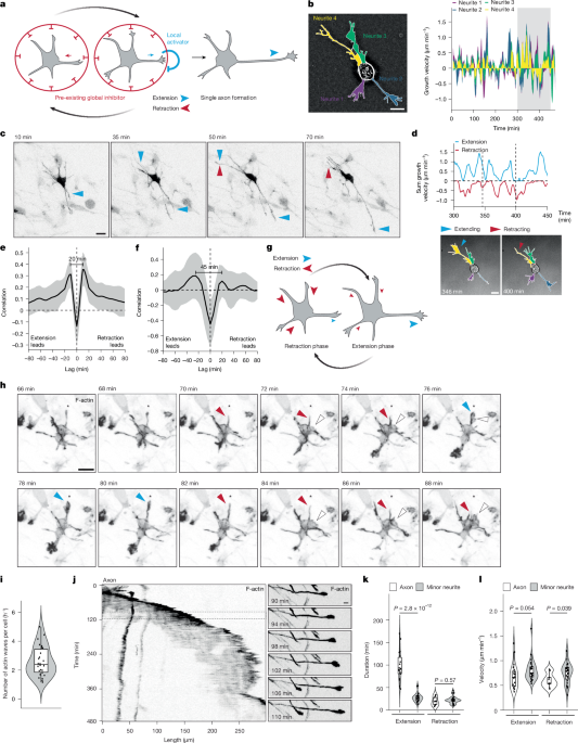
To profile native neurite growth of early-stage neurons, differential imaging contrast images were acquired with a frame rate of 1 frame per min for at least 8 h. To profile filamentous actin fluctuations, we used the live-cell actin probe Lifeact, which has been applied in profiling the dynamics of the leading edge of migrating cells^82,83. As high levels of Lifeact expression affect native actin dynamics and organization and potentially create artefacts in our analyses^84,85, we excluded neurons with high levels of Lifeact from image acquisition.

Neurons expressing Lifeact–mScarlet were acquired with a frame rate 0.25 frames per min for at least 12 h. To profile fluctuations in ARP2/3 and myosin II levels, dual-channel images (Lifeact–mScarlet with ARP3–SNAP-SiR or MRLC–SNAP-SiR) were acquired with a frame rate of 0.2 frames per min for at least 12 h. To profile ARP2/3 and myosin II fluctuations simultaneously, triple-channel images (Lifeact–mScarlet, ARP3–SNAP-SiR and MRLC–mNeonGreen) were acquired with a frame rate of 0.1 frames per min for at least 12 h. To profile subcellular actin (Lifeact–GFP) and microtubule dynamics (EB3–mCherry), the images were acquired with a frame rate of 1 frame per s for 3 or 5 min.

Time-lapse live-cell images of neurons expressing Lifeact–mScarlet and grown in 3D collagen matrix were acquired with a Zeiss LSM880 confocal microscope equipped with a ×20 objective (Plan-Apochromat ×20/0.8 NA M27) as z stacks with a frame rate of 1 frame per 15 min for at least 12 h. Deconvolution post-processing was performed using Zeiss Zen Blue.

Machine-learning-assisted segmentation of brightfield images of neurons

To facilitate extraction of neurite growth profiles from the low-contrast brightfield time-lapse images of neurons, we applied convolutional neural networks to segment the images. The segmentation process defined and distinguished the background, the soma and the neurites from each other.

We performed supervised pixel classification on the basis of machine learning on the time-lapse image stacks. We used the open-source software YAPiC (https://yapic.github.io/yapic/) to train a 2D U-Net (‘unet_2d’ network of YAPiC) with three classes (background, soma and neurites). Training data were collected by manually labelling a subset of time-lapse images with Ilastik software (https://ilastik.org)⁸⁶. A total of 18 images of 10 WT neurons and 19 images of 11 Actr3 KO neurons were labelled. In each image, parts of the soma, parts of the neurites and parts of the background were labelled. To obtain precise segmentation of neurites, in each image, several small sections of neurites at different positions were labelled with the directly adjacent background at pixel-level precision. Larger regions of the background were also roughly labelled, and the soma was labelled more roughly than neurites. More detail is described in documentation available at GitHub (https://yapic.github.io/yapic/example_neurite.html).

The network was trained on an Ubuntu 16.04 workstation equipped with Nvidia TITAN V GPU (12 GB RAM). The labelled data were split into 80% training data and 20% validation data (YAPiC default settings) and trained for 5,000 iterations. Computation time for model training was 5 days. The model with the lowest loss of the validation dataset was applied to all image stacks.

Optogenetic control of ARP2/3 activation with PA-RAC1

We used a previously described PA-RAC1 construct³⁷ for optogenetic experiments with an Andor spinning disk confocal microscope or a Zeiss LSM980 confocal microscope.

The Andor spinning disk microscope was built on an inverted Nikon Eclipse Ti microscope and equipped with a Nikon Perfect Focus system, a Yokogawa CSU-X1 Spinning Disk Unit, a REVOLUTION 500 series AOTF Laser module, iXON EMCCD and Neo Monochrome sCMOS dual cameras and a FRAPPA photobleaching module. The operation and parameter setting were performed with Andor iQ3. We used Nikon Plan Apo ×40 oil objective N.A. 1.4 for light activation and image acquisition.

Neurons expressing mVenus–PA-RAC1 were selected. The photoactivation sites were manually defined as single or multiple spots of 1–4 pixels. PA-RAC1 at the selected sites was sequentially photoactivated with a 450-nm laser controlled by the FRAPPA module. The dwell time of the laser on each pixel was 20 µs and the repetition number was 500. Time-lapse single-plane images of Lifeact–mScarlet were acquired every 10 s before, during and after the photoactivation step. A total of 20 frames were acquired for each session.

For the optogenetic experiments performed with a Zeiss LSM980 confocal microscope, a ×40 objective (Zeiss LD LCI Plan-Apochromat ×40/1.2 Imm Corr DIC M27) was used for photoactivation and Airyscan image acquisition. The photoactivation sites were manually defined as a single region of 4–12 pixels in Zeiss ZEN Black. PA-RAC1 at the selected sites was photoactivated with a 445-nm laser. The spot-bleaching duration was 500 and iteration was 400. Time-lapse single-plane dual-channel Airyscan images (Lifeact–mScarlet and MRLC–SNAP-SiR) were acquired every 20 s before, during and after the photoactivation step. A total of 20 or 30 frames were acquired for each session.

Identical settings for an Andor spinning disk or LSM980 microscope were followed for the control experiment using a photoinsensitive variant of PA-RAC1 (PA(C450M)-RAC1) and for the ARP2/3 suppression experiment using the dominant-negative variant (PA-RAC1(T17N)).

For quantification, the last frame before photoactivation (pre), the last frame of photoactivation (act) and the last frame of deactivation (post) were analysed. To reduce variations caused by heterogeneity of exogenous protein expression and differences in neurite length among neurons, we applied a normalization process. We calculated the direction and the amplitude of changes (intensity and neurite length) relative to the mean by deducting the mean value from the measured values.

Negative-staining electron microscopy

Before cell seeding, Formvar-film-coated 200-mesh Au grids (Gilder Grids) were glow-discharged and coated in 1 mg ml^–1 poly-lysine (Sigma-Aldrich) at room temperature overnight. Subsequently, grids were washed 3 times with PBS, placed in grid holders⁸⁷, transferred into 96-well plates and incubated with conditioned N2 medium at 36.5 °C for 1 h. For seeding of cells onto EM grids, cells were freshly thawed and diluted to achieve a seeding density of approximately two cells per grid square. At 2 h after seeding at 36.5 °C, a medium exchange with fresh conditional N2 medium was performed. Finally, cells were incubated at 36.5 °C for 20 h.

Cells were prepared for negative-staining transmission electron microscopy as previously described⁸⁸, but with minor modifications. In brief, neurons were extracted and mildly fixed in incubating grids in 50 μl droplets of cytoskeleton buffer (10 mM MES, 150 mM NaCl, 5 mM EGTA, 5 mM glucose and 5 mM MgCl₂, adjusted to pH 6.2) containing 0.75% Triton X-100 (Sigma-Aldrich), 0.25% glutaraldehyde (Electron Microscopy Sciences) and 0.1 μg ml^–1 phalloidin (Sigma-Aldrich) for 1 min. For post-fixation, grids were incubated in 50 μl droplets of cytoskeleton buffer containing 2% glutaraldehyde and 1 μg ml^–1 phalloidin for 15 min. Negative staining was performed by dropwise application and immediate blotting of 50 μl total volume of 4% negative-staining solution (10 nm BSA-conjugated gold colloid diluted 1:8 in 4% sodium silicotungstate (Agar Scientific), adjusted to pH 7.0).

Dual tilt axis tomography of negatively stained cytoskeletons was performed on a FEI Tecnai G2 20 operated at 200 kV using SerialEM software⁸⁹. Data were recorded on a FEI Eagle 4k camera at a magnification of ×29,000, resulting in a pixel size of 7.767 Å. Each unidirectional tilt series ranged from −60 to +60° in 1° increments. The defocus was set to −3 μm.

Tilt series alignment and tomogram reconstruction via weighted backprojection was performed in IMOD⁹⁰ by combining the data from two related tilt series obtained around orthogonal axes.

Machine-learning-assisted segmentation and automatic actin filament tracking

To facilitate automatic filament tracking, we applied convolutional neural networks to segment the tomograms and filter out the background and artefactual membrane fragments. We performed supervised pixel classification based on deep learning on all collected EM raw data stacks. We used the open-source software YAPiC (https://yapic.github.io/yapic/) to train a multislice U-Net (‘unet_multi_z’ network of YAPiC) with two classes (background region and actin filament region). Training data were collected by manually labelling a subset of image stacks (3 WT and 3 Actr3 KO stacks, each containing 50–100 slices) with Ilastik software (https://ilastik.org)⁸⁶. Approximately 20% of all pixels in the images were labelled.

The network was trained on a Ubuntu 16.04 workstation equipped with Nvidia TITAN V GPU (12 GB RAM). The labelled data were split into 80% training data and 20% validation data (YAPiC default settings) and trained for 5,000 iterations. Computation time for model training was 5 days. The model with the lowest loss of the validation dataset was applied to all image stacks. This process is described in greater detail in the documentation available at GitHub (https://yapic.github.io/yapic/example_actin_em.html).

The stacks of the actin network model were converted to a mask and applied to the original reconstructed tomograms to remove background and artefacts, leaving the pixels of actin filaments only (Extended Data Fig. 9a). We then performed automatic actin filament tracking with the modified Matlab scripts as previously described^88,91.

Actin filament polarity determination

Analysis of actin filament polarity was done as previously described⁹². In brief, traces of the filaments were interpolated by a 3D spline curve, and subtomograms, including the actin filaments, were extracted along the spline curves. The actin filament in the extracted subtomogram was traced again automatically through correlation with a 3D cylinder. The filament was unbent according to the trace. The unbent filament was 2D-projected onto a plane including the filament axis with the smallest tilt angle against the grid plane. The projected images were analysed using single-particle analysis procedures for filamentous complexes and the filament polarity was determined. The analysis code has been deposited into Zenodo (https://doi.org/10.5281/zenodo.20081075)⁹³.

CK-666-induced neurite retraction

E17.5 mouse hippocampal WT neurons were isolated. After introducing plasmids encoding the indicated reporters (Lifeact–mScarlet, MRLC–SNAP and EB3–mNeonGreen) via electroporation, neurons were cultured on PLL-coated 8-well chamber slides. Time-lapse images were acquired with widefield epi-fluorescence microscopes (DeltaVision RT or DeltaVision Elite, Applied Precision). To have neurons with developed neurites, we started image acquisition 48 h or 72 h after plating for the pre-CK-666 condition. After this session, we pre-mixed the CK-666 stock solution with half of the volume of conditioned N2 medium in the well and then added this mixture back to the original well to achieve a final CK-666 concentration of 150 µM. In this way, we kept the neuron-secreted autocrine growth factors consistent. After 10–15 min of temperature re-equilibration and stage re-focusing, we started another session of image acquisition for the post-CK-666 condition. The acquisition duration was 16–24 h. After this session, cells were washed three times with pre-warmed fresh conditioned N2 medium. After temperature re-equilibrium and stage re-focusing, we started another session of image acquisition for the CK-666-washout condition. Images were deconvoluted with SoftWoRx (v.3.5 or 4.0, Applied Precision).

For investigation of the impact of CK-666 on the lengths of axons and minor neurites of DIV-1 and DIV-3 neurons, DIV-1 (32–36 h after plating) and DIV-3 (80–84 h after plating) neurons were treated with CK-666 (200 µM) dissolved in DMSO. After 12 h of treatment, the treated neurons were fixed with modified PHEM fixative for 20 min and immunostained as described in the above. The neurite tracks and lengths were defined using the Segmented Line of Fiji.

Local perfusion of CK-666 and para-aminoblebbistatin

Hippocampal WT neurons were isolated, and plasmids encoding Lifeact–mScarlet were introduced via electroporation. Neurons were cultured on PLL-coated MatTek 35-mm glass-bottom dishes. Before the experiments, cells were washed twice with pre-warmed HBSS solution and finally with pre-warmed and filtered conditioned N2 medium to avoid blockage of the suction pipette with culture debris. To visualize the application fluid during imaging, FastGreen For Coloring Food (FCF) was diluted in HBSS solution. Then we added the filtered FastGreen FCF HBSS mix to freshly filtered conditioned N2 medium (1:4). Fast Green FCF was imaged during the experiment with far-red excitation. To prepare the application fluid, we mixed the CK-666 and para-aminoblebbistatin stock solution (diluted in DMSO) with the HBSS FastGreen FCF conditioned N2 mix to achieve a final CK-666 concentration of 150 µM and para-aminoblebbistatin of 40 µM. DMSO of the same volume of the added stock solution was used as the control. The application capillary was filled with 10 µl of the application fluid.

For local perfusion, we modified a previously published setup⁹⁴. We used a micromanipulator-controlled application and suction system attached to an Andor spinning disk confocal microscope, configured and controlled as described for the optogenetic control experiments. We used a Nikon Plan Apo ×10/0.45 for positioning the application and suction pipettes in the vicinity of the target neurons and a Nikon Plan Fluor ×40/1.30 for fine adjustment of the pipettes and subsequent image acquisition. To establish local perfusion, we applied positive pressure (3–5 hPa) to the infusion capillary and negative pressure (0.5–1.5 hPa) to the aspiration capillary with two motor-controlled syringe pumps. Once the position and pressure were adjusted to establish a defined local perfusion at the focal plane, the infusion pressure was reduced to stop the outflow. The aspiration pressure was kept constant throughout the experiment.

After placing the target soma or growth cone at the designated local perfusion site, we started image acquisition and local perfusion by initiating the previously established application pressure. After 90 min of local application, the application pressure was released, and the application and suction pipettes were removed. The neuron was imaged for at least 1 h after application. Image analysis was performed using Fiji (v.1.48o).

Quantification of EB3 intensities at growth cones and neurite tips

We manually defined the area of growth cones and neurite tips using the Lifeact channel, which visualizes actin protrusions. We used EB3 intensity to approximate the level of polymerizing microtubules. To reduce interference of photobleaching on measurements, we only analysed the temporal maximum intensity projection of the first 24 frames over 2 min before and after CK-666 treatment.

Neurite tracking, growth profiling and local protein intensity profiling

The procedures below were performed manually with the indicated Fiji plugins or batch-processed with customized ImageJ and Jython macro scripts in Fiji using ImageJ API. The custom ImageJ macros used for generating kymographs, extracting neurite tip positions and protein intensities have been deposited into GitHub (https://github.com/darkbreaker0/IJ_NeuriteGrowthScript).

We used segmented brightfield images of early-stage neurons to define the neurite tracks and to profile native neurite growth. Alternatively, to quantitatively characterize the relationship between neurite growth and local protein fluorescence intensity fluctuations, the actin channel (Lifeact–mScarlet or Lifeact–mNeonGreen) of the images was subjected to neurite track determination and growth profiling. For neurite growth profiling in cortical slice cultures, we used the LYN–mNeonGreen channel. The neurite growth profiles derived from the segmented brightfield and actin fluorescence intensity gave the same neurite growth dynamic.

To define neurite tracks, a temporal projection from the time-series image stacks was generated, which showed the trajectories of neurite growth. Neurite paths were then manually tracked with ‘Segmented Line’. To include the background intensity in the subsequently generated kymograph, the length of the neurite track was at least 10 μm longer than the corresponding neurite. To reduce complexity, neurites were only analysed if they directly originated from the soma such that secondary and tertiary neurite branches were excluded. Following the neurite tracks, the kymographs were generated with the ‘Multi-Kymograph’, with a line width of 3.2 μm used to cover the width of the neurite shaft. This then calculated average intensity across the line width.

To extract neurite growth profiles from the kymographs, a thresholding filter ‘Huang’ was first applied and then the upper threshold value was manually adjusted to define the end positions of the neurite tip. The tip point was defined as the position of the pixel with an intensity above the upper threshold and the longest x axis value. In cases when the bright background speckles interfered with identification of the tip position, the speckles were manually removed from the kymographs beforehand. The end positions of the neurite tip at each time point along the kymograph were defined as the neurite lengths.

To approximate the indicated protein level at the neurite tip, the protein fluorescence intensity was integrated in the 6.2-μm window from the neurite tip at each time point along the kymograph. The protein level at the neurite shaft was defined as the integrated intensity of the whole neurite minus the integrated intensity of the neurite tip. As the integrated intensity at the neurite shaft is proportional to the neurite shaft length (neurite length minus 6.2 μm), the intensity profiles were normalized with the length profiles, which resulted in profiles of actin density at the neurite shafts. To quantify the intensity fluctuations of the indicated proteins at the soma, the soma area was manually defined using ‘Polygon Selection’ and intensity was profiled using ‘Measure stack’.

Cross-correlation of neurite growth dynamics and local protein intensity fluctuations

The extracted neurite growth profiles and the local protein fluorescence intensity profiles were imported and analysed in the integrated development environment RStudio as multiple time-series data registered to the associated neurons (R packages stats::ts and tsibble::as_tsibble). To reduce noise as high-frequency background fluctuations, moving average smoothening (R package forecast::ma) was applied to the multiple time-series data with a window size of 3 for the data with low temporal resolution (profiles derived from cortical slice cultures and triple-channel images) or with a window size of 5 for the data with high temporal resolution (profiles derived from segmented brightfield images and single-channel and dual-channel images).

For the neurite extension–retraction cross-correlation analysis, differential growth profiles of the neurites were generated (R base diff) from the smoothened time-series data (Extended Data Fig. 1d). This differencing step calculated the first derivative (velocity) of the smoothened time-series data over time. Next, at any given time point, from the extending neurites, the positive changes were summed and integrated extension activity profiles were generated (Extended Data Fig. 1d, yellow blocks). Similarly, from the retracting neurites, integrated retraction activity profiles were generated. Pearson’s correlation coefficient between the extension and the retraction was computed as a function of the time lag using the R package stats::ccf. The correlation functions from different cells were pooled, and the averaged cross-correlation function and the standard deviation were calculated (R package rstatix::get_summary_stats).

For the cross-correlation analysis between neurite growth and local protein fluorescence intensity fluctuations, two strategies were applied. The first strategy excluded soma protein intensity profiles and considered one neurite as one sample. It computed the Pearson’s correlation coefficient between the differential growth profile of each neurite and the associated neurite tip or normalized neurite shaft protein intensity differential profiles (R package stats::ccf). The correlation values from all the neurites of different cells were pooled, and the averaged cross-correlation value and the standard deviation were calculated (R package rstatix::get_summary_stats). This strategy is more sensitive in detecting correlations at the individual neurite level.

The second strategy included soma protein intensity profiles and considered one neuron as one sample. The assumption here is that soma protein intensity fluctuations reflect the integration of the overall relationships with every neurite. Consequently, the soma protein intensity fluctuations are less correlated with any one neurite but more with the overall neurite growth and with the overall neurite protein fluorescence intensity fluctuations. To obtain the integrated measurements of all neurites, the measured values of every neurite were summed first (Extended Data Fig. 1d, brown blocks). After moving-average smoothening (R package forecast::ma), the first derivatives of the summed measured values were calculated (R base diff). Pearson’s correlation coefficients of the paired differential profiles from different cells were pooled for the calculation of the averaged cross-correlation function and the standard deviation (R package rstatix::get_summary_stats).

Quantification of ARP3 and MRLC intensities at extending and the retracting neurites

From the neurite growth profiles, we categorized the neurite growth states as extending, pausing or retracting by setting the growth velocity threshold as ±0.02 µm min^–1. The following values were then used for classification: extending, ≥0.02 µm min^–1; retracting, ≤ −0.02 µm min^–1; and pausing, between −0.02 and 0.02 µm min^–1.

For each neuron, the ARP3 and MRLC intensities at the neurite tips of extending, pausing and retracting neurites were calculated. To reduce variations caused by the heterogeneity of exogenous protein expression among neurons and batches of experiments, the averaged ARP3 and MRLC intensities in each neuron was normalized as a Z score with the averaged value of the three growth states.

Neurite length and soma area measurement and categorization of early neuronal morphogenesis stages

The stages of early neuronal morphogenesis are defined by the critical events neuritogenesis and axogenesis. We considered a process longer than 16 µm as a neurite, and a neurite longer than 70 µm and with medial-to-distal accumulation of the axon marker tau as an axon. Therefore, neurons without a neurite longer than 16 µm were categorized as stage 1, neurons with a neurite longer than 16 µm were categorized as stage 2, and neurons with a tau-positive neurite longer than 70 µm as stage 3. Neurons exhibiting multiple axons were also considered stage 3 neurons in spite of aberrant neuronal polarization.

We measured neurite lengths using the Fiji plugin Simple Neurite Tracer⁹⁵ or ‘Segmented Line’. The neurite tracks from the soma to the neurite tips were defined by the microtubules visualized with anti-β3-tubulin. The length of neurite precursors of stage 1 neurons was excluded from neurite length quantifications. For the neurite lengths of stage 2 and stage 3 neurons, we defined the neurites excluding the longest neurite as the remaining neurites. To quantify the soma area, we manually defined the soma contour with ‘Polygon Selection’. The above procedures were performed manually with the indicated Fiji plugins or batch-processed in Fiji using ImageJ API.

Ventricle area and cortical thickness measurement

To quantify the ventricle area of coronal sections of brains from WT and Actr3 KO E17.5 mice, we manually defined the contour of ventricle regions with ‘Polygon Selection’ and measured the area in Fiji.

To quantify cortical thickness, for each coronal section, we measured the thickness of at least eight regions that were randomly selected. The cortical thickness was measured as the shortest distance between the boundary of the ventricle to the contour of the cortex.

The result files were imported in RStudio (v.1.4.1103) and analysed with a customized R script.

Patch-like structure identification tracking, counting and size measurement

To track the movement of ARP3 patches, we applied the Fiji plugin MOSAIC Particle Tracker 2D/3D to detect and track the patches⁹⁶. The following parameters for patch tracking were used: radius, 3–5; cutoff, 0.001; Per/Abs, 0.8–1.5; link range, 1; displacement, 10; dynamics, straight lines.

For the quantification of patch number and patch size, we applied the Fiji plugin ComDet (https://github.com/ekatrukha/ComDet/). The following parameters were used: include larger particles; segment larger particles; approximate particle size, 5–10 pixels; intensity threshold, 5–10; ROI shape, ovals.

The result files were imported into RStudio (v.1.4.1103) and analysed with a customized R script.

Colocalization analysis

To generate the colocalization cross-correlation colour map of selected two channels (ARP3–actin, ARP3–MRLC or MRLC–actin), the images acquired using a DeltaVision microscope were first deconvoluted with SoftWoRx (v.3.5 or 4.0, Applied Precision). To remove the background signals, we applied ‘Subtract Background’ with a rolling radius of 20 pixels. To avoid interference by small, non-specific particles, we applied the ‘FFT bandpass filter’ to filter out objects smaller than 3 pixels. The typical size of ARP3, MRLC and actin patches is larger than 9 pixels for images with a pixel size of 0.065 µm. We analysed the processed images with the Fiji plugin Colocalization Colormap⁹⁷, with the option ‘autothreshold’ checked.

To quantify the colocalization levels of selected two channels (ARP3–actin, ARP3–MRLC or MRLC–actin) at the growth cones and at the soma, the images were processed as described above. The regions of growth cones and the soma were manually defined with ‘Rectangle Selection’. We then applied the Fiji plugin EzColocalization⁹⁸ to quantify the Pearson cross-correlation of the two channels. We selected ‘Costes’ as the autothresholding method.

Quantification of actin branches and orientation in EM tomograms

Branch junctions were manually selected using the IMOD software package. For determination of filament orientation relative to the leading edge, first the contours representing the individual filaments were reordered so that their last point would represent the barbed end, as determined by the polarity analysis. For calculation of angles, filaments were represented by 2D vectors (only considering x and y coordinates) pointing from the first point of the respective contour (pointed end) to the last point of the contour (barbed end), and the leading edge was represented by the 2D unit vector of protrusion rotated 90° in a clockwise direction.

Calculations were performed by applying the following equation in a custom Python3.6 script:

With x and y representing the x and y values of the vectors of the leading edge (LE) or the actin filament (AF). The resulting angles in radians were then transformed to degrees as depicted in the figures.

Statistical information

Data organization and statistical analysis were performed with Excel 2016 (Microsoft), Prism (v.8.0.1 or 9.0.0, GraphPad Software) and with R packages stats, rstatix and ggpubr in R (v.R 4.0.2). The test, the number of data points (n) and the number of independent experiments or biological replicates are described in the figure legends. All tests were two-sided (α = 0.05) and exact P values are reported in the figures or legends. Normality (D’Agostino–Pearson) and homoscedasticity (Bartlett, Brown–Forsythe) were tested before parametric methods.

The following tests were performed in this study: t-tests (Figs. 3i and 4d,r and Extended Data Figs. 3b, 4a,f, 8b,c,k,n,q, 9c,d and 11b,c), Mann–Whitney tests (Figs. 1k,l, 2i, 3h,n, 4h,k,o,p and 5l,m and Extended Data Figs. 2f, 5b,i, 6e,g, 7b,d,f, 8e,j,m and 9i), paired t-tests (Fig. 2d and Extended Data Figs. 3q and 4b–c), paired Wilcoxon tests (Figs. 2h,j,k, 3l and 4f and Extended Data Figs. 2i–k and 11f,i), paired Wilcoxon tests with Holm correction (Fig. 3c and Extended Data Figs. 3n, 5e, 6d,i and 7h,i), one-way ANOVA with Dunnett’s post hoc (Extended Data Fig. 12a), two-way ANOVA followed by Tukey post hoc (Figs. 4j and 5b,j and Extended Data Figs. 8g,i and 12g,j,m,n), two-tailed chi-square test of independence (Fig. 5f,g and Extended Data Figs. 4e and 11g) or Kruskal–Wallis followed by Dunn’s post hoc with Bonferroni correction (Figs. 3g and 5c,d and Extended Data Figs. 3e,f, 4h, 8f,h,p and 12b,d,f,h,l).

Reporting summary

Further information on research design is available in the Nature Portfolio Reporting Summary linked to this article.