An encyclopedia of human enhancer–gene regulatory interactions

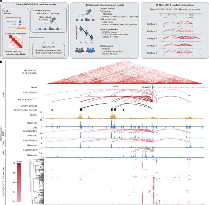
This study did not involve human participants or animal subjects. The combinatorial enhancer perturbation experiment in this study used established cell lines obtained from commercial or publicly available sources. All other computational analyses used publicly available data, and are not considered human subjects research. Refer to the Supplementary Methods for more detailed descriptions of each section in Methods.

Genome build and gene annotations

All coordinates are reported in GRCh38 unless otherwise specified. We used a curated set of 20,678 gene promoters (one per gene symbol), defined as 500-bp regions centred on the RefSeq TSS with the largest number of coding isoforms. Gene symbols were matched to ENSEMBL IDs using the HUGO database⁷² and GENCODE v.29, retaining genes annotated as protein_coding, processed_transcript or lincRNA by GENCODE.

Biosamples and DNase-seq data processing

We computed ENCODE-rE2G and ABC predictions for 1,458 ENCODE DNase-seq experiments covering 369 unique cell types and tissues (Supplementary Table 12). Using the ENCODE API, we downloaded metadata and BAM files for released DNase-seq experiments, filtering for ENCODE4 analysis versions in GRCh38. Sequencing run type (single- or paired-ended) was determined by merging FASTQ metadata with the corresponding BAM file records. Single-ended BAM files were filtered to remove low-quality and multi-mapping reads (samtools view -F 780 -q 30) without PCR-duplicate removal, as duplicate reads are difficult to detect reliably in single-ended high-complexity DNase-seq data. Paired-ended BAM files were obtained as filtered alignments from the ENCODE pipeline, with filtering out low-quality, multi-mapping and PCR-duplicate reads (samtools view -F 1804 -q 30 -f 2 and Picard MarkDuplicates v.1.126). For experiments with mixed run types, only unfiltered alignments from single-ended reads were used. For ENCODE-rE2G^Extended models, additional assay input files were selected manually (Supplementary Table 13).

Defining candidate elements and element–gene pairs

Candidate elements were defined from DNase-seq or ATAC-seq data using MACS2 (–shift −75 –extsize 150 –nomodel) on pooled replicates. After removing blacklisted regions, the top 150,000 peaks by read count were retained and resized to 500 bp centred on peak summits. TSS-centred 500-bp regions for all genes were added and overlapping regions were merged. Elements were classified as promoter (within 500 bp of any TSS), genic or intergenic. Candidate element–gene pairs included all pairs within 5 Mb.

Annotating enhancer–promoter pairs with epigenomic and genomic features

We computed features for each element–gene pair encompassing chromatin state, 3D contact frequency and genomic position (Supplementary Table 2).

Chromatin state

DNase-seq and, where applicable, H3K27ac ChIP–seq read counts were computed for candidate elements, gene bodies and promoters using bedtools coverage, then quantile-normalized to a K562 reference⁹. Cell-type-specific enhancer activity was calculated as the geometric mean of normalized DNase-seq and H3K27ac signals, if included.

Three-dimensional contact frequency

Hi-C contact frequencies were calculated from either cell-type-specific ENCODE Hi-C data or a cell type average Megamap generated by aggregating 65 ENCODE Hi-C datasets (accession ENCSR492BKE). Processing of Hi-C contact matrices included SCALE normalization, interpolation of low-coverage bins using a power-law fit, diagonal replacement, doubly stochastic normalization and pseudocount adjustment⁹. K562 Hi-C loop calls were obtained from the ENCODE portal. CTCF ChIA-PET features (‘Loop Contain’ and ‘Loop Cross’) were computed from PET counts in K562 and GM12878 ChIA-PET data. CTCF contact domains were identified using a two-state hidden Markov model implemented in the sklearn.hmm package for Python 3.8.

Genomic features

Features included distance to TSS, number of intervening TSSs and candidate elements, local element density within 5 kb, enhancer complexity scores⁶, promoter class annotations²⁸ and ubiquitous gene expression²⁸.

Correlation of enhancer–promoter activity across cell types

DNase-seq reads were counted at ENCODE4 candidate cis-regulatory elements (cCREs) and TSSs across 89 biosamples (Supplementary Table 14), normalized per million reads, and log-transformed. Pearson and Spearman correlations and generalized least squares regression coefficients (nlme v.3.1-162) were computed for cCRE–TSS pairs within 1 Mb, using a sample–sample correlation matrix to account for global inter-biosample correlations. An analogous approach was applied to DNase–RNA correlations using 96 polyA⁺ RNA-seq samples (Supplementary Table 15).

Predictive models

ABC model

We applied the ABC model as described previously⁹, with updates including multi-replicate peak calling and activity estimation, ENCODE-recommended MACS2 parameters, hg38 support and a reproducible Snakemake pipeline. ABC scores were computed using DNase-only activity with Megamap Hi-C contact (ABC^{A = DNase, C = Average ENCODE Hi-C}; threshold 0.018) for all 1,458 biosamples, and DNase+H3K27ac activity with cell-type-specific Hi-C (ABC^{A = DNase × H3K27ac, C = ENCODE Hi-C}; threshold 0.027) for K562 and GM12878 (Supplementary Table 1). The updated ABC pipeline is available on GitHub: https://github.com/broadinstitute/ABC-Enhancer-Gene-Prediction.

Other enhancer–gene predictive models

In addition to ENCODE-rE2G and ABC, we applied several other proposed predictive models: EpiMap⁸, EPIraction²⁷, GraphReg¹⁰, Enformer¹¹ and the CTCF loop-CIA model¹⁶. Each was adapted as needed to apply it to ENCODE4 data to generate predictions of enhancer–gene regulatory interactions. Details of each implementation are provided in Supplementary Methods.

Training and applying ENCODE-rE2G

ENCODE-rE2G logistic regression models were trained on a combined CRISPR dataset in K562 containing 10,356 tested element–gene pairs, including 471 positives. For the initial model, 12 features computable from DNase-seq, average Hi-C and genome annotations were used, including both first-order and second-order terms for enhancer activity and 3D contact frequency to capture possible non-linear effects; for ENCODE-rE2G^Extended, 45 features available in K562 and GM12878 were used (Supplementary Tables 3 and 8). Features were variance-stabilized (log[|x| + 0.01]) before fitting unregularized logistic regression models. Performance was evaluated using hold-one-chromosome-out cross-validation, holding out each of the 23 chromosomes (1–22 and X) as the test set in turn. To apply the models to new cell types, we generated cell-type-specific feature tables as described above and applied a model trained on all 23 chromosomes to each candidate element–gene pair. A Snakemake workflow for applying trained ENCODE-rE2G models to new datasets is available on GitHub: https://github.com/EngreitzLab/ENCODE_rE2G.

Collection of published predictions and baseline predictors

We collected enhancer–gene predictions from ten previously published methods (Supplementary Table 1), lifting predictions from hg19 to GRCh38 where necessary. Details of each collected method are provided in Supplementary Methods. Baseline predictors were generated for 1,458 biosamples based on distance to TSS, nearest expressed gene and variants thereof, using both ENCODE DNase-seq narrowPeak (DNase hypersensitivity sites) and candidate elements defined here (ABC) (Supplementary Table 16). For 24 selected biosamples, additional baseline predictors were computed including distance to the gene body, nearest TSS or gene within 100 kb and DNase-seq signal (and H3K27ac signal for 20 biosamples) at the element multiplied by 1/distance. Classification thresholds for all models were set at 70% recall on the combined CRISPR data (Supplementary Table 1).

Creating the combined K562 CRISPR training dataset

We collected three published CRISPR enhancer screen datasets in K562 from Nasser and colleagues⁶ (mostly CRISPRi-FlowFISH), Gasperini and colleagues¹⁸ (Perturb-seq) and Schraivogel and colleagues²² (TAP-seq). For Perturb-seq and TAP-seq data, we developed a unified analysis pipeline. Unique molecular identifier counts were normalized for cell-level size factors (excluding the top 10% expressed genes), log-transformed and differential expression was tested using MAST⁷³ (v.1.20.0) between perturbed cells and sampled control cells, with Benjamini–Hochberg FDR correction (less than 5%). Statistical power was estimated by simulation-based analysis using negative binomial count distributions with gene-specific mean and dispersion parameters estimated by DESeq2 (ref. ⁷⁴) (v.1.34.0), incorporating guide–guide variability in knockdown efficiency (σ = 0.13, learned from FlowFISH data⁹) across 20 simulation replicates. For the Gasperini dataset, guide-to-element assignments were re-computed using BLAT alignment, and candidate elements were defined from the top 150,000 K562 DNase-seq peaks. For the Schraivogel dataset, genes within the same genomic region (chr. 8 and chr. 11) were tested for each targeted element. Datasets were filtered to retain element–gene pairs with distances of 1 kb–1 Mb from TSS, excluding elements overlapping GENCODE v.29-annotated promoters or target gene bodies. Negative pairs required ≥80% power to detect a 15% decrease in expression. Negatives in the Nasser dataset were filtered for at least 80% power to detect a 25% decrease in expression based on the provided power analysis. Duplicate pairs across datasets were resolved by prioritizing significant results or, when significance status matched, highest statistical power at 25% effect size.

Creating the combined held-out CRISPR dataset

Eight CRISPR perturbation screens across five cell types were collected for held-out benchmarking: Perturb-seq experiments in K562 (refs. ^31,32,33), DC-TAP-seq in K562 and WTC11 (ref. ⁷⁵) and CRISPRi-FlowFISH in K562 (ref. ³⁵), HCT116 (ref. ³⁴), GM12878 (ref. ⁶) and Jurkat⁶. Perturb-seq datasets were reprocessed uniformly with standard cell quality filtering (unique molecular identifier counts, mitochondrial transcript fraction and gene detection thresholds) and guide validation through BLAT alignment to hg38, retaining only guides mapping uniquely with 100% sequence similarity. Top 150,000 candidate elements were defined from K562 DNase-seq data using the ABC pipeline⁹. Differential expression was performed using SCEPTRE (v.0.10.0) with high multiplicity of infection settings, union guide integration, two-sided testing and 10% FDR. The above-described power analysis was adapted for SCEPTRE, testing effect sizes of 2–50% across 100 replicates per effect size. DC-TAP-seq datasets⁷⁵ were obtained with published SCEPTRE-based results and power estimates; FlowFISH results and power analyses were obtained from the original publication⁶.

To create the final held-out dataset, duplicates within the same cell type were resolved (prioritizing significant results, then highest power), and pairs present in the training dataset were removed. Pairs were filtered by genomic location using GENCODE v.29 annotations, removing elements overlapping any annotated promoter (1 kb upstream of TSS) or the target gene body. Negatives were filtered for at least 80% power at 15% effect size (Perturb-seq/DC-TAP-seq) or 25% (FlowFISH), and positives required more than 5% effect size for Perturb-seq/DC-TAP-seq. Positives lacking H3K27ac signal (CTCF, H3K27me3 or no H3K27ac categories) were removed to focus on enhancer-mediated regulation.

Annotating CRISPR elements with chromatin categories

Tested elements were annotated using H3K27ac, H3K27me3 and CTCF ChIP–seq peaks and quantitative H3K27ac RPM in the corresponding cell types (BAM files and peak calls from the ENCODE portal; additional ChIP–seq performed for Jurkat). Elements were categorized hierarchically based on H3K27ac peak overlap and RPM percentile as High H3K27ac, H3K27ac, CTCF, H3K27me3 or No H3K27ac (see Supplementary Methods for details).

Calculating direct and indirect effect rates of CRISPR experiments

Indirect effect rates were estimated empirically for K562, WTC11 and uniformly reprocessed Perturb-seq datasets^18,31,32,33, by testing each distal element perturbation against 100 randomly selected genes on other chromosomes, restricting to genes present in the cis discovery analysis to ensure comparable expression distributions. The dataset-specific indirect rate was calculated as the proportion of significant trans-acting tests using the nominal P value cutoff corresponding to the FDR threshold of each dataset in the cis discovery analysis. The direct effect rate as a function of distance to TSS was calculated by subtracting the distance-independent indirect rate from the observed positive hit rate, computed in 50-kb distance bins within 1 Mb of the TSS. To predict the direct effect rate for any distance, a power-law function was fitted to model direct effects versus distance using only bins with positive direct rates. For datasets where indirect rates could not be empirically estimated, the average empirical rate was used. The probability of each element–gene pair representing a direct effect was computed as:

CRISPR benchmark

Predictive models were benchmarked against both training and held-out CRISPR datasets. For each model, CRISPR elements were overlapped with prediction elements based on genomic coordinates (matched by gene symbol), with scores aggregated using predictor-specific functions (sum or max, Supplementary Table 1) when several predictions overlapped a single CRISPR element. Elements without overlapping predictions were assigned the minimum possible score. AUPRC and precision/recall at 70% recall were computed (ROCR v.1.0-11), with 95% confidence intervals estimated by bootstrapping (10,000 iterations; boot v.1.3-28.1). Significance of pairwise comparisons was calculated by bootstrapping delta metrics and computing two-sided P values by inversion of confidence intervals (boot.pval v.0.7.0). No correction for multiple testing was applied unless specified otherwise. Weighted precision-recall curves were computed using the yardstick package (v.1.2.0), weighting each pair by its estimated probability of being a direct regulatory effect (Supplementary Methods 22).

GWAS benchmark

We assessed whether predicted enhancers were enriched for fine-mapped GWAS variants and could link those variants to probable causal genes. Fine-mapping was performed on 94 UK Biobank traits (application 31063) using SuSiE on up to 361,194 people of white British ancestry with variants meeting INFO > 0.8, minor allele frequency > 0.01% and Hardy–Weinberg equilibrium P > 1 × 10⁻¹⁰. Associations were estimated using BOLT-LMM (quantitative traits, inverse rank transformed) or SAIGE (binary traits), controlling for principal components, sex, age and related covariates. SuSiE allowed up to ten causal variants per region (± 1.5 Mb around lead variants), pruning credible sets at r² > 0.25 and excluding the MHC region (chr.6, 25–36 Mb) and credible sets with variants having fewer than 100 minor allele counts. Noncoding credible sets were defined as those not containing coding or splice-site variants (within 10 bp of a splice site).

Enrichment was calculated as the fraction of noncoding variants (PIP > 0.1) in merged enhancer sets divided by the fraction of common and low-frequency 1000 Genomes variants in enhancers. Heritability enrichment was assessed using S-LDSC^76,77, computing both enrichment and standardized effect size (\(\tau \)*) for each annotation. For gene-linking evaluation, we identified 560 noncoding credible sets near exactly one gene carrying an independent coding variant (protein-truncating or damaging missense, PIP ≥ 0.5), after deduplication across genetically correlated traits, using 197 blood-trait loci as the primary benchmark. The combined ENCODE-rE2G ∩ PoPS score was computed by intersecting the top two ENCODE-rE2G gene predictions per biosample with the top two PoPS³⁸ gene predictions per variant within a 1-Mb window.

eQTL benchmark

We benchmarked models using GTEx³⁶ v.8 eQTL variants fine-mapped with SuSiE⁷⁸ (PIP > 0.5), filtered to variants in credible sets with corresponding HGNC gene symbols and linked to genes expressed above 1 transcript per million in the relevant tissue. Variants were filtered to distal noncoding regions by excluding coding sequences, untranslated regions, splice sites (within 10 bp of intron–exon junctions) and promoters (±250 bp from TSS) of protein-coding genes. GTEx tissues were matched to prediction biosamples for each model (Supplementary Table 5), with 13 tissues represented across all models used for primary benchmarking. Enrichment was defined as the fraction of eQTL variants overlapping predicted enhancers divided by the fraction of distal noncoding 1000 Genomes single nucleotide polymorphisms in predicted enhancers. Recall was computed as the fraction of eQTL variants overlapping predicted enhancers linked to the correct eGene, and enrichment-recall curves were constructed by evaluating 50–100 threshold quantiles per model.

Assaying enhancer activity

To evaluate different activity measurements, ABC scores were computed for all element–gene pairs using 523 one-dimensional chromatin experiments in K562 (Supplementary Table 17). Each assay was substituted for DNase-seq in the activity calculation, with read-depth normalized signal (DNase-seq) or fold-change over control (ATAC-seq, ChIP–seq) bigWig files downloaded from the ENCODE portal. K562 ENCODE Hi-C was used for contact frequencies in all models.

Linking variants to genes

The ENCODE-rE2G ∩ PoPS prediction was generated by intersecting the top two genes from ENCODE-rE2G scores for a peak overlapping a variant with the top two genes from PoPS³⁸ in a 1-Mb window. PoPS prioritizes genes for a disease by training a model to predict MAGMA⁷⁹ (v.1.08) gene scores using 57,543 gene-level functional features (bulk and scRNA-seq, biological pathways and PPI networks) in a leave-one-chromosome-out framework, making the combined score disease-specific. For each of 352 cell types and 76 diseases, the top two ENCODE-rE2G genes per biosample were intersected with the top two PoPS genes. For comparison, OpenTargets L2G > 0.5 maps were curated for 1,512 study IDs (Supplementary Table 10), and an OpenTargets ∩ PoPS combination was similarly constructed.

Combinatorial enhancer perturbations at the MYC locus

A CRISPRi-FlowFISH screen was conducted to perturb all pairs of seven previously characterized MYC enhancers²⁶ in K562 cells. A library of 10,080 paired single guide (sg)RNA vectors was designed using a lentiviral dual-promoter system (hU6 and mU6), targeting seven enhancers (e1–e7), the MYC TSS, two adjacent cCREs and one negative control element (NS1), with eight sgRNAs per element paired in an all-by-all fashion in both orientations, plus 80 additional vectors to calibrate recombination rates. sgRNAs were selected from previous experiments²⁶ or GuideScan (CFD ≥ 0.2, efficiency ≥ 50), with 12 additional sgRNAs targeting safe harbour regions⁸⁰.

The library (Twist Bioscience) was transduced into doxycycline-inducible dCas9-KRAB K562 cells at multiplicity of infection of approximately 0.1 (55 million cells per replicate, greater than 500-fold coverage) across two biological replicates. K562 cells were purchased from ATCC and engineered previously to express KRAB-dCas9 (ref. ⁹). After puromycin selection and doxycycline induction (48 h), cells were processed for FlowFISH using probe sets for MYC and RPL13A across seven technical replicates, sorted into six fluorescence bins on a BD Influx sorter. sgRNA pairs were amplified and sequenced on an Illumina NextSeq with custom primers. Guide pair abundances were quantified using Bowtie 2 (ref. ⁸¹) and Samtools⁸², and mean fluorescence estimated by maximum likelihood⁹. Effect sizes were corrected for background signal (1.57-fold correction⁹), quality-filtered (≥200 cells per guide pair per bin), and refined by selecting the two highest-effect sgRNAs per element before aggregation. Significance was assessed by two-sided one-sample t-tests across technical replicates. Observed dual perturbations were tested for non-additive effects using a two-sided t-test against 0 on the interaction term of a linear model (Effect = E1 + E2 + E1 × E2).

Enhancer synergy analyses

To assess whether enhancer effects sum to more than 100%, we analysed 20 comprehensive CRISPRi tiling experiments^6,9,26, retaining enhancers with significant negative effects (adjusted P (P_adj) < 0.05) not overlapping promoters, with exceptions for two PVT1 promoter regions shown to act as MYC enhancers²⁶.

To examine whether enhancer perturbations affect nearby enhancer activity, we performed H3K27ac ChIP–seq following CRISPRi perturbation of seven individual MYC enhancers and one negative control element in K562 cells as described previously⁸³ (two biological replicates per gRNA, 3–4 ChIP–seq experiments per element, 16 negative control experiments). Fold-change in H3K27ac reads per million was computed at each ABC candidate enhancer. We also analysed published datasets: CRISPRi–H3K27ac data from Fuentes and colleagues⁵¹ targeting long terminal repeats in NCCIT cells (625 uniquely mappable long terminal repeat regions); H3K27ac chromatin QTLs from Delaneau and colleagues⁵³ and CRISPR-deletion H3K27ac data from Huang and colleagues⁵².

Cell line authentication and mycoplasma contamination

All cell lines used in experiments performed as part of this study were authenticated through analysis of epigenetic data. All cell lines were tested for mycoplasma contamination.

Data visualization

Plots were generated in R (v.4.2.0) using the following packages: tidyverse (v.1.3.2), ggplot2 (v.3.5.1), ggextra (v.0.10.1), ggpubr (v.0.6.0), ggcorrplot (v.0.1.4.1), ggrastr (v.1.0.2), cowplot (v.1.1.3), Gviz (v.1.42.0), GenomicInteractions (v.1.32.0).

Locus plots in Figs. 1a, 3e and 4a, Extended Data Fig. 6 and Supplementary Fig. 1 were created using the GViz (v.1.42.0) and GenomicInteractions (v.1.32.0) packages for R (v.4.2.0). Locus plots for Fig. 5b, and Supplementary Figs. N1.3 and N5.2 were created using the IGV genome browser⁸⁴ (https://igv.org/app). Arcs in all locus plots show predicted E–G regulatory interactions above the chosen model thresholds.

Reporting summary

Further information on research design is available in the Nature Portfolio Reporting Summary linked to this article.