


Bats
Fifteen adult male Egyptian fruit bats (Rousettus aegyptiacus) were included in this study for neural recording experiments (weight, 160–200 g). Information on individual bats is summarized in Extended Data Table 1. All experimental procedures for the neural recordings were approved by the Institutional Animal Care and Use Committee of the Weizmann Institute of Science. An additional 12 bats were included in a behavioural-control experiment in a smaller setup, without neural recordings (see below).
Behavioural setups for neural recordings
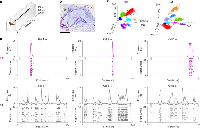
Four different behavioural setups were used in this study, shown in Extended Data Fig. 1a,b. All of the setups used tunnels with identical cross-section shape, with a width of 2.3 m and maximal height of 2.35 m (ref. 12), with uniform illumination (5 lux). Details on individual bats in each setup are found in Extended Data Table 1.
-
(1)
Linear flight sessions in long tunnel: ten of the recorded bats flew back and forth in fixed-size linear tunnels of lengths 200 m or 130 m, shuttling between two landing balls positioned at the two ends of the tunnel (Extended Data Table 1, bats 1, 3 and 7–14; Extended Data Fig. 1a). Note that these lengths are rounded: The 200-m tunnel had an effective length of 194 m, and the 130-m tunnel had a length that varied between 129–134 m across sessions.
-
(2)
Flight sessions in short linear segment: four bats were recorded in an additional separate session in which they flew in a short segment of the tunnel: either 6 m (bats 1, 14 and 15) or 15 m (bat 4). These segments were blocked with opaque curtains or solid blocks at both ends.
-
(3)
Landmark perturbation: two bats (bats 2 and 4) performed two recording sessions, separated by a short sleep session of 5–10 min. A single prominent landmark was moved 7.5 m between session 1 and session 2 (the positions of the perturbed landmark are shown in Extended Data Fig. 1b (orange triangles); photograph of the perturbed landmark is shown in Extended Data Fig. 1d). The perturbed landmark was moved daily between the exact same two positions for these two bats.
-
(4)
Switching between multicompartment session and linear-flight session in long tunnel: four bats (bats 2, 4, 5 and 6) performed two recording sessions, separated by a short sleep session. In the first recording session (session 1) the bats flew in the large multicompartment tunnel (Extended Data Fig. 1b, top); 193 m length) between 3 landing balls positioned at the 3 ends of the tunnel. Rewards were given equally after landing at each landing ball, and there were therefore no correct or incorrect choices in this paradigm. In the second recording session (session 2), the junction leading to the two short compartments was blocked with a black opaque curtain, and a landing ball was positioned just before the curtain, leaving a 180 m straight tunnel for the bats to fly back and forth between the two landing balls (Extended Data Fig. 1b, bottom). Note that the 180-m tunnel had an effective length of 174 m.
Each behavioural session started and ended with sleep sessions (each sleep session lasting 5–10 min). For the sleep sessions the bat was placed inside a small covered cage, which was positioned in a quiet location inside the tunnel.
In all of the experiments, human experimenters were sitting at the ends of the tunnel (beyond the landing balls). The humans were outside of the area in which the bats were flying.
Training of bats and recording sessions
All 15 bats were initially pretrained for a few days in a flight-room or in a short segment of the tunnel (6 m or 10 m), with the aim of getting used to handling by humans and learning to perform direct flights between two landing balls. Then, 12 bats were further trained for an average of 3 weeks in the 200 m tunnel (8 bats) or in the 180 m multicompartment environment (4 bats) to fly continuous long flights. After this training, the neural recordings began. Two additional bats were recorded in the 130 m tunnel: Neural recordings in these bats were conducted from the first day of exposure to the long tunnel; we note that in our previous study12, we did not find any change in neural coding in CA1 along days in these two bats. Three of these 14 bats were also neuronally recorded in shorter tunnels (6 m or 15 m; see Extended Data Table 1). One additional bat (bat 15) was neuronally recorded only in the short 6 m tunnel.
After training, all of the bats were implanted with a microdrive for electrophysiological recordings in the dorsal hippocampus (see below).
Animal localization system
We tracked the position of recorded bats using wireless ultra-wideband radio-frequency localization tags (weight 6.6 g, including battery; BeSpoon), which received and transmitted signals to an array of ground-based antennas that were distributed around the tunnel, as was done in our previous work12 (14–40 ground-based antennas, depending on the experimental setup). This localization method yielded a good precision of 5–10 cm in the longitudinal axis (x) and lateral axis (y) of the tunnel. Specifically, we used two setups: The first setup (all of the bats recorded in the 200 m or 130 m tunnels; Extended Data Table 1) had 14 ground-based localization antennas, which yielded a localization precision of 10 cm in x and y. The second setup (all of the bats recorded in the 180 m tunnel and the multicompartment experiments) had 40 localization antennas with a large vertical span, which yielded a localization precision of 5 cm in x and y, and a precision of 20 cm in the vertical axis (z). The position of the bats was acquired at a sampling rate of between 12.8 and 18 Hz. The localization system and the neural recording system were synchronized using a non-periodic sequence of TTL pulses (with temporal precision of <1 ms).
Surgery and neural recordings
All of the surgical procedures were performed as described previously12,57. In brief, after completion of training, bats were implanted with either a 4-tetrode microdrive (weight, 2.1 g; Neuralynx) or a 16-tetrode microdrive (weight, 3.4 g; modified from ref. 60), loaded with tetrodes, with each tetrode constructed from four strands of insulated wire (17.8-μm diameter platinum-iridium wire). Tetrodes were gold-plated to reduce the wire impedance to 0.3 MΩ (at 1 kHz). The microdrive was implanted above the right dorsal hippocampus (3.0–3.6 mm lateral to the midline and 5.8 mm anterior to the transverse sinus that runs between the posterior part of the cortex and the cerebellum); the craniotomy was then covered with an inert silicone elastomer (Kwik Sil or Kwik-Cast). During the implantation surgery, we used an injectable anaesthesia cocktail composed of medetomidine (0.08 mg per kg), midazolam (2.5 mg per kg), fentanyl (0.025 mg per kg) and ketamine (17 mg per kg) (or, in some bats, medetomidine (0.25 mg per kg), midazolam (2.5 mg per kg) and fentanyl (0.025 mg per kg)), and added supplemental injections as needed, on the basis of the bat’s breathing and heart rate (as measured using an SA Instruments model 1025T Small Animal Monitoring System). The microdrive was attached to the skull with bone screws, using a layer of adhesive (Super-Bond C&B) followed by dental acrylic. We attached the ground wire from the microdrive to a bone-screw that touched the dura in the skull’s frontal plate.
After surgery, the tetrodes were slowly lowered toward the CA1 pyramidal layer; positioning of tetrodes in the layer was provisionally performed on the basis of the presence of high-frequency field oscillations (ripples) and associated neuronal firing. After recording cells in the CA1 cell layer, in five of the recorded bats we further lowered some of the tetrodes to reach the CA3 cell layer, and subsequently conducted recordings simultaneously in CA3 and CA1 (Extended Data Table 1). For each bat, one tetrode was left in an electrically quiet zone and served as a reference, and the remaining tetrodes served as recording probes. The tetrodes’ exact recording location was later verified histologically (Fig. 1b and Extended Data Fig. 5b).
During recordings, a wireless neural-recording device (neural logger; 16 channels or 64 channels, Deuteron Technologies) was attached to a connector on the microdrive. Signals from all channels were amplified (×200) and bandpass filtered (1–7,000 Hz), and were then sampled continuously at 31.25 or 32 kHz per channel, and stored on board the neural logger. During subsequent processing, the neural recording was further high-pass filtered with a 600 Hz cut-off for spikes, creating a spike bandwidth of 600–7,000 Hz and then a voltage threshold was used for extracting 1 ms spike waveforms.
Histology
At the end of recordings, the bats were anaesthetized, and electrolytic lesions (DC positive current of 30 μA for 15 s duration) were made in a subset of the tetrodes, to facilitate the reconstruction of tetrode positions. The bat was then given an overdose of sodium pentobarbital and, with tetrodes left in situ, was perfused transcardially using PBS followed by 4% paraformaldehyde or 4.5% Histofix. The brain was removed and post-fixed. Thin coronal sections were then cut at 30 or 40 μm intervals on a freezing microtome. The sections were Nissl-stained with cresyl violet and were photographed to determine the locations of tetrode tracks in dorsal CA1 or CA3 (Fig. 1b and Extended Data Fig. 5b). Positions of tetrode-tracks were then mapped onto coronal plates of a stereotaxic brain atlas of the Egyptian fruit bat61, and were then projected onto a 3D reconstruction of CA1 and CA3 cell layers, which we prepared on the basis of our stereotaxic brain atlas. Finally, we used these projections to estimate the tetrode-track position along the longitudinal axis and proximodistal axis of CA1 and CA3 (Extended Data Fig. 5; both the proximodistal axis and longitudinal axis are curved anatomical axes within the 3D space of the bat brain; we therefore estimated the distances along these curved axes). In the analysis in Extended Data Fig. 5, we did not include tetrodes with poor histology, for which we were able to localize the tetrode tracks to CA1 or CA3 but were not able to localize with sufficient accuracy the exact tetrode location within each subregion (this excluded data from 3 out of the 14 bats recorded in the long tunnels).
Spike sorting
Spike-sorting procedures were identical to those described previously12,57. In brief, spike waveforms were sorted manually using Plexon Offline Sorter, on the basis of their relative amplitudes on different channels of each tetrode. Data from all of the behavioural sessions and sleep sessions from the same recording day were spike-sorted together. Well-isolated clusters of spikes were manually selected, and a refractory period (<2 ms) in the interspike-interval histogram was verified. Spike sorting was performed in consecutive time windows to allow for drift correction of the spike clusters. We included only neurons that were stably isolated throughout the recording. We further analysed only putative pyramidal cells with mean firing rate <5 Hz, which met behavioural-coverage criteria as described below for the different behavioural setups. A summary of the number of cells analysed for each type of behavioural session is provided in Extended Data Table 1.
Statistics
For all of the pairwise comparisons, we used two-tailed (two-sided) statistical tests, with a probability threshold of α = 0.05. Correlations were based on Spearman’s correlation coefficient (two-tailed test), unless noted otherwise. We used the Wilcoxon rank-sum test to compare distribution medians, and the two-sided Kolmogorov–Smirnov test to compare distribution shapes. To determine the significance of place tuning, we compared the real data with shuffled data (see below). No power analysis was used to predetermine the sample size.
Extracting flights
Flight behaviour was analysed separately for the experiments in the linear tunnels (130 m and 200 m: Extended Data Fig. 1a) and for the experiments in the multicompartment and 180 m tunnel (Extended Data Fig. 1b), as follows:
In the linear tunnels, the bat flight behaviour was mostly restricted to a 1D narrow horizontal corridor at the middle of the tunnel12. Thus, for these linear environments, all of the analyses and statistical tests were performed strictly on the basis of 1D firing-rate maps (projections on the long axis of the tunnel), as described previously12. In brief, location data were first processed to remove outliers (we removed datapoints that were outside the tunnel’s walls (>80 cm), or data with velocity higher than 20 m s−1). We then linearized the data by projecting the valid positional data onto the long 1D axis of the tunnel (the tunnel’s ‘backbone’, which was measured using the radio-frequency localization tag). We then filled short gaps where localization data were missing. We used linear interpolation to fill gaps up to 1.5 s, only if flight speed was stable during the gap. This gap-filling procedure yielded a maximal error of no more than 25 cm on average, as tested by introducing simulated gaps in real data that had no gaps. Finally, the 1D positional data were upsampled to 100 Hz. Directional flight epochs were detected as periods during which the bat’s speed was >1 m s−1 and reached a peak speed >4 m s−1, without changes in flight direction.
In the multicompartment environment, to capture the 2D shape of the environment, we used 2D raw positional data from which we extracted the 2D flight speed. Thus, to define flight epochs, we increased the flight speed threshold to >2 m s−1, while maintaining the same criterion for peak speed >4 m s−1 and requiring the absence of changes in flight direction (note that typical flight speeds were actually much higher than 4 m s−1)12. We then extracted for each flight its start and end positions, and assigned these positions to one of the environment’s compartments: long, straight or turn compartments (compartments are defined in Extended Data Fig. 10b). Next, we linearized each flight to a 1D axis, while keeping the identity of the flight’s start and end compartments. Gaps in the flights were filled in a manner similar to that described above for the linear flights. As in this multi-compartment setup we had an improved localization precision of 5 cm, it enabled us to fill gaps up to 5 s (instead of 1.5 s); only gaps that occurred in the long part of the tunnel (away from the junction) were filled, provided that the flight speed was stable during the gap, and that the bat’s wingbeat-rate was highly stable (as assessed using an on-board accelerometer). Similar to the linear flight setup, the gap-filling procedure was tested by introducing simulated gaps in real data which had no gaps, and it yielded a maximal error of no more than 25 cm on average. Finally, the 1D positional data were upsampled to 100 Hz.
Computing firing-rate maps
Firing-rate maps were constructed for flight periods only—separately for the two flight directions. For the multicompartment experiments we also separated the data on the basis of the flight start and end compartments. To compute 1D firing-rate maps, we counted the number of spikes and the time spent in each spatial bin (20-cm bins). Bins with time spent <0.75 s per metre were discarded. We smoothed both the spike-count and time-spent 1D map with a Gaussian kernel (σ = 2.5 bins, namely 0.5 m), and then divided, bin by bin, the smoothed 1D spike-count by the smoothed 1D time spent, to produce a firing-rate map. We included for further analysis only sessions with (1) more than 10 flights per direction and (2) valid firing-rate map with no gaps for at least 100 m. For the short tunnels (6 m and 15 m) we used 1D speed threshold of 1 m s−1, threshold for peak speed of 2 m s−1, smaller spatial bins of 10-cm and a smoothing kernel of σ = 2 bins, namely 0.2 m. We also analysed U-turns, as shown in Extended Data Fig. 14.
Quantifying spatial coding, definition of place cells and defining place fields
To quantify the spatial coding of firing-rate maps, we used the spatial information (SI) index, measured in bits/spike (Fig. 2d): \(\mathrmSI\left(\frac\mathrmbits\mathrmspike\right)=\sum _ip_i\left(\fracr_i\barr\right)\log _2\left(\fracr_i\barr\right)\), where ri is the firing rate of the cell in the ith bin, pi is the probability of the bat to be in the ith bin, and \(\barr\) is the overall mean firing rate of the cell. Place cells in CA1 and CA3 were classified as significant place cells only on the basis of the linear flight data (using the linear tunnels and the blocked session, excluding the multicompartment session) if they met the following criteria: (1) significant spatial information compared to spike shuffles (>99% of shuffles): to shuffle the spike trains, we rigidly and circularly shifted in time the spikes of each flight, using a uniform random shift; the value of the shift differed randomly between individual flights, so each shuffle consisted of a unique set of temporal shifts that differed randomly across flights. We performed 1,000 such random shuffles for each neuron. (2) Spatial information was >0.25 bits per spike. (3) A cell emitted a minimal number of spikes in-air per flight direction during the entire session: ≥50 spikes in the 130 m and 200 m tunnel experiments; and ≥20 spikes in the blocked session of the multicompartment experiment (we used here a lower spike-count threshold because the two behavioural sessions resulted in fewer straight-flight trials per session); we also required ≥20 spikes in the short tunnel experiments, where the reduced time in-air limited the spike count. (4) The cell had at least one significant place field, as described next.
To detect place fields, we used the same algorithm as we used previously12 and applied it to both CA1 and CA3 data. (1) First, we extracted local peaks in the firing-rate map, with a peak-rate of >1 Hz. (2) To remove small local peaks ‘riding’ on a large field, we searched for shallow ‘dips’—that is, cases in which the dip between two adjacent peaks was >50% of the firing rate of the larger peak—and then disregarded the lower peak. (3) We then defined the boundaries of the field as follows: we identified the zone covering 20% of the peak firing rate of that place field. Then, to overcome the smearing caused by the smoothing of the firing-rate map, we defined the field size as the 5–95% percentile of the positions of the spikes that occurred inside the 20% zone. (4) Field stability criterion: we required at least 10 different laps inside the place field, out of which there were at least 5 different laps with spikes inside the place field, or 20% of the laps with spikes, whichever is larger. (5) Field significance criterion: to capture clear distinct fields, we treated a place field as significant only if it had significant spatial information in its local area, near the place field. To quantify this, we looked at the area surrounding the field (specifically, the field itself plus 50% of the field’s size on each side). Focusing on this local area around the place field, we calculated the spatial information for the real spikes and compared it to 1,000 shuffles (same rigid shuffling as above), and considered the field to be significant only if it had spatial information of >95% of the shuffles in this constrained local area.
For each neuron we computed four indices: (1) spatial information, in bits per spike, as defined above (Fig. 2d). (2) Total coverage of all of the fields, defined as the sum of all field sizes per direction, normalized by the length of the flight track (Fig. 2e). (3) Sparsity (Fig. 2f), defined as \(\frac\langle r_i\rangle ^2\langle r_i^2\rangle =\left(\sum p_ir_i\right)^2/\sum p_ir_i^2\), which is bounded between 0 and 1, with low values indicating high spatial selectivity and sparser coding. (4) Map correlation, an index of map stability, computed as the Pearson correlation coefficient between maps constructed separately for the first half versus second half of the session (Fig. 2c) or for odd versus even flights (Extended Data Fig. 4c). These four indices were computed separately for each flight direction.
All of the comparisons of spatial coding in CA3 versus CA1 in Fig. 2 were performed using only data from the linear flight sessions (using data from the linear tunnels (200 m and 130 m) and from the session in which the tunnel was blocked (180 m linear tunnel); here we excluded the data from the multicompartment session).
Generating model maps and decoding simulations
For the decoding simulations (Fig. 3a–c), we created populations of neurons with simulated place fields, using the multifield multiscale encoding scheme described before12 for CA1 maps, and a single-field encoding scheme for CA3 maps. We used a maximum-likelihood decoder to study the decoding accuracy implied by these two encoding schemes, for populations of CA1 neurons and CA3 neurons. Decoding was done with an integration time window of 500 ms.
Encoding
In our simulations, the environments had a 0.2-m resolution (0.2-m bin size); the same binning as was used to analyse the real data. We varied the size of the environment, L, between 20 m and 1,000 m. The neurons had rectangular fields, did not fire outside their fields, and fired at a fixed rate m0 within their fields (with Poisson statistics).
CA3 scheme
For each neuron, we picked a single field, with a field location that was sampled from a uniform distribution over the environment of length L (measured in metres). The field size was sampled randomly from a gamma distribution (which is very similar to a log-normal distribution12), with a shape parameter α and a scale parameter θ, which were calculated from the experimental distribution of CA1 and CA3 field sizes for the 200 m and 180 m environments (L = 200 metres) (α = 3.46 and \(\theta =1.46\times \sqrtL/200\,\textmetres\)). The square-root scaling of the field-size distribution with the environment size L is consistent with field-size distributions measured at multiple environment sizes (Fig. 2h and Extended Data Fig. 3h).
CA1 scheme
For each neuron, the field sizes were randomly chosen from a gamma distribution identical to the distribution used for the CA3 scheme. The number of fields was chosen such that the cumulative coverage of all of the fields together reached \(0.139\times L\times \sqrt200/L\,\rmmetres\). The pre-factor 0.139 represents the neurons’ average coverage at the 200 m environment size in our experiments (Fig. 2i and Extended Data Fig. 3i). Field locations were randomly distributed along the environment, with no overlaps. The square-root scaling of the coverage with the inverse of the environment size is consistent with our recordings at multiple environment sizes (Fig. 2i).
We denote each neuron’s spatial selectivity map by \(f_i^a(x)\), where i is the neuron index (i = 1, …, N), and a is the scheme index (a = CA3 or CA1). \(f_i^a(x)\) is equal to 1 if the neuron has a field in position x and 0 if it does not, that is, the field shapes in our model were taken to be rectangular.
Generating spike counts
We assumed that the animal starts each simulation trial at a position x = x0, and flies at speed v = 8 m s−1 (the typical empirical flight-speeds) for a time interval Δt = 500 ms. The expected spike count of the neuron during that trial is given by:
$$m_i=m_\undersetx_\oversetx_+v\Delta t\int f_i^a(x)\rmdx,$$
where m0 is the expected spike count if the animal spent the entire interval within a field. We used m0 = 5 in all our simulations (taken together with the integration time window of 500 ms, this gives a typical in-field firing rates of 10 Hz). The actual spike-count in each trial was drawn from a Poisson distribution with rate mi and is denoted below as ni.
Maximum-likelihood decoding
We computed the log-likelihood of each simulated neuron’s spike count, and summed it over the N neurons:
$$A_\mathrmML(x)=\mathop\sum \limits_i=1^Nn_i\log [m_\,f_i^a(x)]-m_\mathop\sum \limits_i=1^Nf_i^a(x)$$
where the first term corresponds to a sum of the spatial tuning of all neurons, weighted by their activity. The second term corresponds to the correction for unequal coverage in different locations. The decoded location was then taken as the one that maximizes AML(x).
Figure 3a,b show results from 105 simulation-trials generated by drawing random field locations 100 times, then drawing random spike counts from the Poisson distribution 20 times, and then performing decoding at 50 equally spaced locations x0 spanning the entire environment (100 × 20 × 50 = 105). Figure 3c shows results from 5,000 simulation trials for each value of N. Note that the probability of catastrophic decoding errors (errors larger than 5% of the environment size) shown in Fig. 3b is not a monotonic function of environment size—it first decreases and then increases again. This non-monotonic behaviour arises because catastrophic errors were defined as a fixed percentage of the environment size (namely 5%), whereas the spatial coverage of the simulated firing-rate maps scaled with the square root of the environment size (a choice that was motivated by the experimental data (Fig. 2i)). The interaction between these differently scaled quantities resulted in the observed non-monotonic dependence of catastrophic error probability on environment size.
Decoding using matched firing rates between CA1 and CA3
We controlled here for the possibility that the better decoding performance in CA1 stems from higher mean firing rates in that region compared with CA3. Notably, CA1 neurons show higher mean firing rates because they have more fields and larger coverage than CA3 neurons, and not because of differences in the in-field firing rates (Extended Data Fig. 4a). We controlled for the mean firing-rate differences by performing similar decoding simulations as in Fig. 3a–c, but after matching the mean firing rate for the maps in CA1 and CA3 (Extended Data Fig. 7c–f). Specifically, we kept the parameters for CA1 maps as before (and therefore the decoding performance for CA1 was as in Fig. 3a–c), whereas, for CA3 maps, we matched the mean firing rate to the mean firing rate of CA1 maps, by multiplying the parameter m0 by the ratio between the average coverage of CA1 maps and the average coverage of CA3 maps. Note that this ratio depends on the environment size L, but for all values of L the ratio was greater than 1, resulting in higher peak firing rate in CA3 neurons compared with CA1 neurons.
Target-map learning simulations and quantifying the learning time
For the target-map learning simulations (Fig. 3d–f and Extended Data Figs. 8, 9g and 13g), we implemented node perturbation (NP) and weight perturbation (WP) learning algorithms to obtain the synaptic weights that minimize the reconstruction error of a target CA1 map \(f_i^\mathrmCA1(x)\) for CA1 neuron i, based on banks of CA3 maps \(f_k^\mathrmCA3(x)\). We considered banks of N = 200 independently sampled CA3 maps—namely, 200 CA3 inputs to a CA1 neuron—for which we systematically varied the number of fields nf that each CA3 map had (nf = 1, …, 6 fields; k = 1, …, 200 CA3 maps; different 200 maps for each value of nf; note that 200 maps in CA3 provide sufficient coverage for each CA1 map to yield all possible fields locations, without any empty spaces). We assumed that synaptic weights Uik are learned to minimize the reconstruction error. Specifically, given the target map, the input maps, and a set of synaptic weights \(U_ik\), the squared location-specific reconstruction error was defined as
$$\epsilon _i^2(x)=\left[f_i^\mathrmCA1(x)-\mathop\sum \limits_k=1^NU_ikf_k^\mathrmCA3(x)\right]^2.$$
In NP, following ref. 37, in each iteration t, we perturbed the output neuron (node) by adding to its response a random number \(\xi _i(t) \sim \)\(\mathcalN(0,\sigma _\mathrmNP^2)\). The squared location-specific reconstruction error including the node perturbation is then
$$\epsilon _i,\mathrmNP^2(x)=\left[f_i^\mathrmCA1(x)-\left(\mathop\sum \limits_k=1^NU_ikf_k^\mathrmCA3(x)+\xi _i(t)\right)\right]^2.$$
The NP learning rule for the synapses between CA3 neuron k and CA1 neuron i is implemented as
$$\Delta U_ik^\mathrmNP(t)=-\eta _\mathrmNP\xi _i(t)\mathop\sum \limits_x=1^L(\epsilon _i,\mathrmNP^2(x)-\epsilon _i^2(x))f_k^\mathrmCA3(x).$$
In WP, the weights are perturbed with synapse-specific noise \(\xi _ik(t) \sim \mathcalN(0,\sigma _\rmWP^2)\) rather than perturbing the output. Now the squared error is
$$\epsilon _i,\mathrmWP^2(x)=\left[f_i^\mathrmCA1(x)-\mathop\sum \limits_k=1^N(U_ik+\xi _ik(t))f_k^\mathrmCA3(x)\right]^2,$$
and the WP learning rule is implemented as
$$\Delta U_ik^\mathrmWP(t)=-\eta _\mathrmWP\xi _ik(t)\mathop\sum \limits_x=1^L(\epsilon _i,\mathrmWP^2(x)-\epsilon _i^2(x)).$$
We ran each simulation for 1,000 time-steps for each spatial bin. We used the parameters \(\sigma _\rmNP=1\) and \(\sigma _\rmWP=0.2\). The learning rate parameter \(\eta \) was optimized for single-field maps in CA3 (nf = 1), to yield the fastest learning, namely the fastest monotonic decrease of the average reconstruction error. We then used a grid search over different values of η and nf, and confirmed that, similar to the birdsong literature36, the optimal learning rate η is inversely proportional to the number of CA3 fields nf (in the birdsong study, η scaled inversely with the number of bursts in a song); specifically, we found \(\eta _\mathrmNP=5\times 10^-6/n_\rmf\) and \(\eta _\mathrmWP=5\times 10^-6.5/n_\rmf\). We therefore scaled η inversely with nf in our simulations. For each learning algorithm and each number of fields of CA3 maps, we learned separately the weights to reconstruct 500 target maps in CA1 (namely, i = 1, …, 500). As the learning process of a single map can be noisy, we smoothed the learning curve as follows. For each specific target error, we drew randomly 250 of the 500 target maps, averaged those 250 learning-curves and computed the learning time from this averaged learning curve; this process (of drawing 250 maps and computing the learning-time) was repeated 200 times and the resultant learning time—shown in Fig. 3e and Extended Data Fig. 8—was computed as the median of these 200 learning-times.
Note that our theoretical model is deliberately simplified and does not account for contributions from other regions, such as inputs from CA2 or the entorhinal cortex into CA1. This simplification was motivated by our previous finding showing independent dynamics of different place fields of the same CA1 neuron12. This previous finding is more consistent with synaptic plasticity that potentiates or depresses independent inputs from single-field neurons12, such as inputs from the sparse CA3 neurons (Figs. 1 and 2), rather than inputs which have multiple fields, such as inputs from grid cells in entorhinal cortex, where single neurons have multiple fields62. In other words, our previous findings suggested that the most plastic inputs into CA1 are coming from CA3 neurons with single fields, rather than from entorhinal cortex; this is why we ignored the entorhinal cortex in our model. Nevertheless, even when we incorporated into the model additional non-plastic inputs to CA1 (non-CA3 inputs, see the next paragraph), the sparse CA3 inputs provided an advantage in the learning speed of CA1 output maps compared with dense CA3 inputs (Extended Data Fig. 8c).
Learning with input from both CA3 and EC/CA2
In these simulations (Extended Data Fig. 8c), the target map was set to fi(x) + zi(x), where fi(x) is the original target map and zi(x) arises due to non-plastic spatial input representing an additional external input into CA1, such as from the entorhinal cortex (EC) or from CA2 (this input is constant throughout the learning, but different from one position to the next). For each spatial bin x, zi(x) is sampled from a Gaussian distribution with mean 0 and variance ϕ(1 − ϕ), independently of every other bin, where ϕ is the average coverage of all CA1 target maps. As fi(x) for every x is a binary variable, its variance is ϕ(1 − ϕ). Thus, setting the variance of zi(x) to ϕ(1 − ϕ) ensures that the magnitudes of the learned component and the external component are equal.
Learning after a local perturbation to an already-learned environment
In these simulations (Fig. 3f and Extended Data Figs. 8d and 9g), the local perturbations were performed by increasing the firing rate of target CA1 maps by a factor of 4 in an 8-m region within the map, and learning the weights that best reconstruct this modified map. For each map these simulations were initialized using the final value of the synaptic weights obtained from the original learning simulation described above.
Learning of context-dependent maps
In these simulations (Extended Data Figs. 8e and 13g), each neuron in CA1 received inputs from a set of CA3 neurons, each of which had a context-dependent spatial representation. Specifically, each CA3 neuron represented the animal’s location based on two maps generated independently, corresponding to two different contexts (for example, flights from two different start locations: retrospective coding). Each CA1 neuron was required to produce two distinct output target maps, one for each context, using a single set of synaptic weights linking input and output maps. The synaptic weights were updated according to the node-perturbation learning rule, with a training protocol that alternated between the two contexts.
Firing-rate map changes with respect to landmark perturbation
Bats flew in two behavioural sessions, and one prominent landmark was moved by 7.5 m between the two sessions, keeping in place all of the other landmarks (Fig. 4a,c: the two locations of this landmark are marked with dashed and solid orange lines). This manipulation was performed in two bats, during 27 and 18 recording days in bats 2 and 4, respectively. In all of these recording days, in the first behavioural session the landmark position was x = 70.5 m, and in the second session the landmark was moved to position x = 78 m. The two sessions differed not only by the perturbed landmark location but also in the environment’s structure: in the first session, the environment included two short 10-m segments at one end of the 180-m tunnel, while in the second session, these segments were blocked, resulting in a linear 180-m tunnel (Extended Data Fig. 1b). Importantly, the two environments were identical in the first 180 m, with the only difference being the perturbed landmark in positions between 70.5–78 m, which was more than 100 m away from the blocked short segments (the block was positioned at x = 180 m). Nevertheless, to isolate the effects of the perturbed landmark from any potential effects of prospective or retrospective coding at the far end of the tunnel (close to x = 180 m; Fig. 5), we limited our analysis of the landmark-perturbation effects (Fig. 4) as follows. For forward flights (eastward), we analysed the first 140 m of the tunnel (x = 0–140 m) and, for returning flights (westward), we analysed the last 100 m of the flight trajectory, corresponding to the first 100 m of the tunnel (x = 0–100 m). These areas were chosen for the analysis on the basis of the range of prospective and retrospective coding effects (prospective coding was overall weak (Fig. 5e, left), and retrospective coding (for returning flights) was mostly limited to the eastern half of the tunnel, x > 100 m (Fig. 5e, right)—which is why we focused the analysis of landmark-perturbation on the area x = 0–100 m, which was unaffected by retrospective coding). Only days with a minimum of 10 flights in each of the two sessions and valid firing-rate maps of at least 100 m were included for further analysis (n = 45 experimental days). Firing rate versus position for individual flights was calculated with 1-m spatial bins and smoothed with a Gaussian kernel (σ = 2.5 bins, namely 2.5 m). The firing-rate values of all of the flights within each spatial bin were compared between the two behavioural sessions (t-test with Bonferroni correction for the number of spatial bins: we corrected for the number of non-zero firing-rate bins that were compared between the two sessions). Significantly changed positions in the tunnel were defined as two or more consecutive spatial bins which were significant on the basis of the t-test, and were located within the position range as described above (Fig. 4a, orange dots above the firing-rate maps; population: Fig. 4c, grey and purple bins). The number of changes across place cell maps per spatial bin were compared to a shuffle distribution, in which the significantly changed bins of each map were shuffled with a random rigid circular shift across all of the bins of the map that had valid behaviour and non-zero firing rates. We performed 1,000 such shuffles (1,000 sets of these random shifts) and calculated in the same way as for the original map the distribution of changed bins as a function of position along the tunnel. Only one spatial bin had a larger number of changed firing-rate bins as compared to 99% of the shuffles; this significant bin was located close to the perturbed landmark position, and this spatially focused change occurred only in the CA1 maps (Fig. 4c, top left). The over-representation of firing-rate changes near the perturbed landmark was further assessed using a binomial test, under the assumption of a uniform probability of change along the tunnel. This probability was defined as the number of observed changes across all locations divided by the number of spatial bins eligible for comparison (that is, bins with non-zero spiking activity in at least one of the two sessions). The test revealed a significantly higher than chance number of changes near the perturbed landmark in CA1 (Fig. 4c, top left, two spatial bins (asterisks)). In both the binomial and shuffle tests, no significant changes were found in the population of CA3 maps (Fig. 4c, top right).
To account for the different numbers of place cells in CA1 and CA3, we matched (subsampled) the number of CA1 cells to that of CA3 (n = 22) and repeated the analysis over 1,000 subsampling repetitions. In 95% of these repetitions, place cells in CA1 still showed a greater number of firing-rate changes near the perturbed landmark than place cells in CA3. Furthermore, the over-representation of changes near the perturbation site was statistically significant (on the basis of the binomial test) in 45% of the subsampling repetitions (45% at the α = 5% chance level for an individual test is highly significant: P < 10–300, population-wise binomial test).
Population vector correlations for prospective and retrospective coding
For multicompartment recording sessions, we constructed population vectors from the firing-rate maps of the entire place cells population (separately for each bat, pooled over all of the recording days of the bat). These population vectors were computed separately for four different flight types (Fig. 5a, dark blue and red arrows): (1) forward flight direction ending in the straight compartment (to-straight) or (2) ending in the turn compartment (to-turn); and (3) returning flight direction starting from the straight compartment (from-straight), or (4) starting from the turn compartment (from-turn). The population vectors were then smoothed by averaging over a sliding window of 10 m (boxcar smoothing), with 0.2 m steps, and then the firing-rate map of each cell was normalized separately to a firing-rate range of 0–1, by dividing the smoothed map by its peak firing rate. Then, for each spatial bin (each position), we calculated the Pearson correlation between pairs of population vectors: (1) correlations between to-straight versus to-turn flights, which quantifies prospective coding in the neuronal population (Fig. 5e, left, black); (2) correlations between from-straight versus from-turn flights, which quantifies retrospective coding in the neuronal population (Fig. 5e, right, green); (3) correlations between opposite flight directions, which served as a control, capturing the baseline near-zero correlation due to the global remapping that is known to occur in 1D environments between two opposite movement directions12,31 (Fig. 5e, lower grey curves; shown is the average per spatial bin of the correlation of to-turn versus from-turn and correlation of to-straight vs. from-straight, both of which are for flights in opposite directions); and (4) correlations between maps for odd and even flights in the same directions, which served as another control, capturing the high correlations expected for stable tuning (Fig. 5e, top grey curves). The population vector correlations were plotted as a function of position (Fig. 5e and Extended Data Fig. 13a). Correlations in the short compartments were calculated by correlating the data for the turn and straight compartments; the low correlations there reflects remapping. Confidence intervals for the correlation values were determined by randomly drawing 50% of all of the neurons without replacements, with 1,000 repetitions (25–75% of correlation values across repetitions for each position; plotted as green, black and grey shading, for the retrospective, prospective and control population-vectors, respectively, in Fig. 5e and Extended Data Fig. 13a).
This analysis was done fully in three bats: bat 2 (Fig. 5e (top) and Extended Data Fig. 13a (rows 1 and 5), bat 5 (Extended Data Fig. 13a (row 3); a small number of neurons were recorded in this bat), and bat 6 (Extended Data Fig. 13a (row 4); recordings in CA1 only). Bat 4 allowed only partial analysis because it always flew stereotypically from the straight 10-m tunnel to the long tunnel, and never turned left from the turn-compartment to the long tunnel, which did not permit analysis of retrospective coding, but only of prospective coding (this bat is shown in Extended Data Fig. 13a, row 2).
Variability of retrospective coding
Variability of retrospective coding. To quantify the variability of retrospective coding (high variability means low robustness), we analysed the population-vector correlation curves for the retrospective case (green curves for CA1 in Fig. 5e and for CA3 in Extended Data Fig. 13a, rows 5–6). Variability was computed separately for populations of CA1 and CA3 place cells. To allow direct comparison between CA1 and CA3, both cell populations were randomly subsampled to include an equal number of cells (n = 50 place cells; 1,000 repetitions). For each of the 1,000 subsamples, the variability of the population-vector retrospective curve was quantified as the median of the s.d. of this curve in 10-m spatial windows, therefore reflecting local fluctuations in the population-vector correlation curve on a 10-m scale. The distribution of variability values across subsampling iterations was summarized using box plots, comparing CA1 versus CA3 (Fig. 5g, left, and in Extended Data Fig. 13e,f, left). To further examine the contribution of multi-field coding to robustness, the analysis was repeated after restricting the dataset to neurons with single spatial fields (in both CA1 and CA3; right panels in Fig. 5g and in Extended Data Fig. 13e,f).
Prospective and retrospective place-field classification
To analyse significant prospective/retrospective changes in individual place fields (Extended Data Fig. 13c,d), we performed the following analysis on the long arm of the tunnel (180 m). Place fields were detected as described above (see the ‘Quantifying spatial coding, definition of place cells and defining place fields’ section). The fields were detected separately for firing-rate maps for the four conditions: to-straight, to-turn, from-straight, from-turn. Owing to significant differences in behaviour within the 20 m closest to the junction (positions between x = 160 and 180 m), all place fields in this region were excluded from the analysis in Extended Data Fig. 13c,d (this range is marked by peach shading in Fig. 5e and Extended Data Fig. 13c-d; on average, across recording sessions and bats, there were significant changes in trajectory and speed for 22 m after the turn (x = 158–180 m)). For positions 0–160 m, place fields were classified as significant prospective or retrospective fields if they met the following two criteria: (1) firing rate during flight passes inside the place field was significantly different for straight-compartment versus turn-compartment flights (two-sided t-test over all of the individual flights of a session). (2) No difference in behavioural variables: y position (flight position along the lateral axis of the tunnel width), z position (flight height) and flight speed were all not significantly different for straight-compartment flights versus turn-compartment flights that passed inside the place field (t-test for each variable separately; 228 fields out of total of 1,668 fields were excluded from this analysis due to significant differences in behaviour in either of these 3 behavioural variables). These requirements ensured that the firing-rate changes inside the place field were genuinely representing effects of the future or past compartment—namely prospective or retrospective coding—and were not due to behavioural differences in flight trajectory or speed. In cases in which one or more behavioural variables was significantly different inside the place field, between flights ending in the straight and turn compartments, a matching procedure was performed, such that only flights that overlapped in y-position, z-position and speed were included as valid flights for the firing-rate comparison. If, after removal of unmatched flights, the firing rate inside the place field was significantly different for straight-compartment versus turn-compartment flights, then the place field was considered as a significant prospective or retrospective field. All statistical comparisons required a minimum of five valid flights passes through the examined place field in each of the flight types (5 flights after flight removal based on matching of the behaviour). We then classified all of the place fields in the multicompartment behavioural session, which were located at the long compartment of the tunnel (0–160 m), to one of four categories: (1) prospective fields; (2) retrospective fields; (3) non-significant prospective or retrospective fields; or (4) fields with non-valid behaviour (a field was classified in this fourth category if within the field any one of the behavioural variables was significantly different between flight types, or if there were fewer than 5 flight passes in one of the flight types). The percentage of significant prospective and retrospective fields versus position in the tunnel was plotted in Extended Data Fig. 13c, separately for CA1 and CA3 place cells. We also computed a contrast index for prospective, retrospective and non-significant fields, as follows (Extended Data Fig. 13d): \(\mathrmContrast\,\mathrmindex=\frac\mathrmFR_a+\mathrmFR_b\), where FRa is the mean firing rate inside the field for flights starting or ending in the turn compartment, and FRb is the mean firing rate for flights starting or ending in the straight compartment.
Echolocation analysis in the long tunnel
To assess whether differences in echolocation can explain retrospective coding (Fig. 5), we performed an analysis of echolocation click rate in the multicompartment experiments (Extended Data Fig. 14a–e). To detect the echolocation clicks, we used an ultrasonic microphone on board the neural logger. In all of the experimental sessions in the long tunnel, we recorded simultaneously the audio signal, together with the neuronal signal (both were saved on the neural logger, synchronized at a microsecond precision). The audio signal was filtered (in hardware on the logger) between 4–40 kHz, and was recorded at a 100 kHz sampling rate. Detection of echolocation clicks emitted during flight was then performed offline similarly to ref. 57. We first further high-pass-filtered the audio signal at 10 kHz. We then normalized the signal by its mean absolute deviation (MAD) over the entire session—transforming the amplitude to an SNR. We then used an amplitude threshold of 50 MADs (that is, SNR = 50), which detected clicks reliably. We also applied several additional criteria for click-detection, as described in detail in ref. 57.
To exclude the possibility that the observed strong retrospective coding after 90° turns (Fig. 5) is directly linked to the observed increase in echolocation clicks—that is, that the retrospective coding reflects direct sensory or motor neuronal responses, or changes in attention levels (as echolocation click-rate is known to be a proxy of attention57)—we used U-turns as a control. The rationale is that the motor action of mid-flight U-turns is at least as challenging as 90° turns. For each experimental day we calculated the echolocation click-rate maps for individual flights, in the same way, with the same parameters and bin-sizes as for the neural firing-rate maps, and compared the echolocation click-rate in 90° turns versus U-turns. We found that echolocation click rates were similar between the two types of turn flights (90° turns and U-turns; Extended Data Fig. 14d), which suggests that a similar sensory input and similar attention levels are required for 90° turns and U-turns—yet the neural representations after 90° turns and U-turns were very different (Extended Data Fig. 14h–j). We therefore conclude that differences in echolocation or attention level cannot explain the strong retrospective coding that we found in the hippocampus (Fig. 5)—rather, the retrospective coding probably reflects memory of where the bat came from.
Behavioural control experiments and echolocation analysis in small L-shaped setup
As a further behavioural control for the potential origin of retrospective coding (Fig. 5), we also performed a separate experiment to assess the possible effects of echolocation beam aim (direction of the echolocation beam in space; Extended Data Fig. 14f,g). The purpose of this additional control experiment was to further examine the relationship between echolocation and turning behaviour during flight. To this end, we performed a separate set of behavioural experiments on an additional cohort of bats without neural recordings. These bats were flying in a separate small L-shaped environment that was constructed with similar dimensions to the turn in the large tunnel (Extended Data Fig. 14f). These behavioural control experiments were performed at Johns Hopkins University and were approved by the Institutional Animal Care and Use Committee of Johns Hopkins University. The walls of this L-shaped setup were made from cardboard and were lined with felt to minimize echo reflections that could interfere with sonar signal analysis. Twelve Egyptian fruit bats (6 males, 6 females) participated in these control experiments. The bats were released from both ends of the tunnel. Opening or closing the central door at the L-junction prompted bats to make different navigational choices: fly straight or perform 90° turns or 180° turns (U-turns). The conditions were pseudorandomized across bats and trials. Echolocation clicks were recorded with a 32-channel microphone array consisting of 32 electret condenser microphones (D500X Ultrasound Detector, Pettersson Elektronik). The sensitivity of each microphone was calibrated using a precision microphone (40DP 1/8′′, GRAS, and 7016 1/4′′, ACO Pacific). Signals picked up by each microphone were band-pass filtered between 10 and 100 kHz, amplified with a gain of 10× (SBPBP-S1, Alligator Technologies) and recorded at a 250 kHz sampling rate.
Bat flight trajectories were recorded using a motion-capture camera system with 15 cameras (Vicon T40 and T40S), operating at 200 fps. Three reflective markers were affixed to a lightweight crown that was glued on the bat’s head. These markers served as reference points for reconstructing 3D flight paths63. Moreover, three markers were placed on each of the microphones in the room to capture the microphones’ positions and directions. Infrared cameras (Phantom Miro 310, Vision Research) were used to record the bats’ flight behaviour and confirm their position in the tunnel.
Sonar gaze deviation and click-rate patterns were compared across different navigation trajectories: straight flights, 90° turns and 180° turns (U-turns). Sonar gaze deviation was defined as the angular deviation between each echolocation click’s directional vector63 and the bat’s instantaneous flight direction, with 0° representing alignment between the two. Instantaneous flight direction was calculated as the vector between the bat’s position in the current video-frame and its position in the subsequent video-frame. A three-point boxcar filter was applied to each click’s sonar gaze measurement, and the absolute value of this smoothed average was used as a measure of the sonar gaze deviation.
Sonar gaze deviation and click-rate were then measured relative to the time of the bat’s turn. For each flight trajectory, the moment of maximum curvature was identified and set as time zero (turn time). All clicks were then aligned relative to this timepoint. The median sonar-gaze deviation across all clicks that occurred within a time window of 1 s centred around time zero was compared between U-turns and 90° turns, and showed similar sonar gaze deviation values between the two trajectory types (Extended Data Fig. 14g). This result further supports the finding that the echolocation behaviour of Egyptian fruit bats is comparable between U-turns and 90° turns in the main experiment (Extended Data Fig. 14d). Thus, the fact that we observed strong retrospective coding after the 90° turns (Fig. 5), but not after the U-turns in the long multicompartment tunnel (Extended Data Fig. 14h–j), suggests that the retrospective effect is not due to the motor action of turning, or attention levels, but is instead due to the past trajectory or context (the originating compartment).
Additional discussion
Previous theoretical studies had suggested that dense and sparse codes offer both computational advantages and disadvantages. Dense distributed codes—whereby each neuron represents many inputs (locations) and, consequently, many neurons are active at any moment—allow efficient coding, whereby a large number of different stimuli can be represented by a small number of neurons51,64. Sparse codes—whereby each neuron represents only a few inputs, and where, consequently, only a small fraction of neurons are active at any moment—allow higher memory capacity, efficient use of associative memory for storage and retrieval, and faster learning compared with dense codes36,64,65. Furthermore, studies of artificial neural networks have demonstrated additional advantages of sparse coding. When sparse neural representations are enforced in the hidden layers of a network through regularization, this sparsification reduces computational complexity, helps avoid overfitting and enhances the network’s generalization ability66,67. Our results suggest that the hippocampus may use the advantages of both dense and sparse coding: Our spatial decoding analysis showed that the CA1 dense code allows high-efficiency positional encoding (Fig. 3a–c), and our neural network simulations showed that the CA3 sparse code allows faster learning of spatial maps in CA1 (Fig. 3d–f). Such rapid learning of CA1 maps is consistent with experimental findings on rapid emergence of place fields in CA1, supported by mechanisms of behavioural timescale synaptic plasticity41,68.
Sparse representations can have multiple manifestations. We found here that spatial maps in CA3 are much sparser than those in CA1 within the same environment, in the sense that place cells in CA3 have much fewer fields than in CA1. Although previous studies of place cells in rodents have not found such large differences in spatial coding between the CA3 and CA1, it has been observed that CA3 cells are less likely to be active in each environment than CA1 place cells, that is, a smaller fraction of CA3 cells participates in spatial encoding for a given space3,11,27,69. Even stronger population-level sparsity was reported in the dentate gyrus70,71,72. In our study, we also observed stronger population-level sparsity in CA3 than in CA1 in bats (Fig. 2j). This form of sparsity in the rodent CA3 and dentate gyrus has been a key ingredient for several computational models of hippocampal function72,73,74,75, which highlights again the theoretical advantages of this architecture. We propose that the sparse-to-dense coding transformation between CA3 and CA1 that we identified here may constitute one stage in a broader sparse-to-dense information-processing hierarchy, extending from the sparsest region, the dentate gyrus, through CA3, to CA1, and possibly ending with the highly dense subiculum10,28,76,77,78,79. A similar proposal can be found in the literature28. We view our model focusing on the CA3-to-CA1 connectivity as a first approximation for the hippocampal computation, and suggest that future neural recordings should be performed in large environments from all of these subregions, as well as from entorhinal cortex and CA2, to elucidate the contribution of these areas to hippocampal spatial computations.
Finally, we found in the landmark perturbation experiment (Fig. 4) that in response to a local spatial perturbation in the environment, CA1 neurons—but not CA3 neurons—showed over-representation of firing-rate changes around the perturbed landmark. We note that this difference in responses between CA1 and CA3 place cells may be consistent with previous rodent studies showing that CA3 place fields typically tile environments rather uniformly, whereas CA1 place fields tend to accumulate around locations associated with learning, such as reward sites80,81 (although we note that we did not observe accumulation of place fields but rather accumulation of changes in fields near the perturbation area).
Reporting summary
Further information on research design is available in the Nature Portfolio Reporting Summary linked to this article.

