


Materials
The first stage of this paper, the construction of the EUROPE-IGM-ATLAS, relies on harmonized cross-country individual-level survey data. The second stage, an application of our database in which we use the indices to investigate the relationship between intergenerational mobility and innovation, relies on aggregate datasets from several sources discussed below. These include proxies for innovation and localized controls for initial economic conditions.
To estimate intergenerational mobility of education, we use 11 waves of the ESS conducted between 2002 and 2023. The ESS is a representative cross-national survey in which 40 countries have participated in at least one round since the 2002/2003 wave. Importantly, it includes questions about the level of education and retrospective questions on parental education, therefore enabling us to measure intergenerational mobility while avoiding the bias associated with selectivity in co-residency samples49. We pool all survey waves and apply survey design weights, normalizing the weights to make them consistent across waves30. Furthermore, we restrict our sample to respondents who were at least 22 years old, and were therefore likely to have completed their education, when the survey was conducted. The analysis could be sensitive to this restriction if individuals had not yet completed their educational career. Suitable robustness checks imposing different age restrictions (for example, older than 25) yield no significant changes in the resulting estimates.
We operationalize our definition of migrants in two ways; (1) first-generation migrants, who were not born in their country of residence; and (2) second-generation migrants, those with an indirect migration background either because their parents were first-generation migrants or because they do not possess the citizenship of their country of residence. We use these definitions to construct three versions of our indices: (1) excluding first-generation migrants only; (2) excluding both first- and second-generation migrants; and (3) including migrants. As migration could be endogenously related to both human capital allocation and economic performance within regions50, in our main application, we use the version of our indices obtained by excluding first-generation migrants, giving us a total sample size of 257,919 individuals. Estimations based on the two alternative samples (that is, the sample excluding individuals with a migration background and the one including both natives and migrants) yield consistent results (Supplementary Table 10). In general, see Supplementary Table 11 for clarification on database versioning.
To compute estimates at the subnational level, we use information about the region of residence of ESS respondents (that is, their geographical location of residence in adulthood at the time the survey was conducted). Regional information in the ESS is recorded using country-specific administrative codes that correspond to varying levels of the NUTS (Nomenclature of Territorial Units for Statistics) classification system. Participating countries provide regional identifiers at different hierarchical levels, with some countries coding at NUTS 1, some at NUTS 2, and others at NUTS 3. Moreover, there have been temporal changes in NUTS boundaries, particularly at smaller spatial scales. This creates substantial heterogeneity in regional granularity both within and across survey waves.
To achieve consistent cross-national and cross-temporal comparability, we implement a harmonization procedure. We compute estimates at both the NUTS 1 and NUTS 2 levels where possible. Thus, for countries who code at the NUTS 3 level, we aggregate upward. For regions where NUTS 2 boundaries changed substantially between survey rounds, we do not provide NUTS 2 level estimates, instead further aggregating to the more stable NUTS 1 classification to preserve temporal consistency. The version of the NUTS that serves as the basis of our harmonized definition of regional unit is the 2016 version, with the exception of Poland—which is included based on the 2008 NUTS boundaries due to regional divisions in later versions of NUTS. Our definition of regional boundaries is further augmented by the addition of non-EU countries, such as Serbia, Kosovo, Montenegro and so on. A cartographical depiction is shown in Supplementary Fig. 4.
The NUTS classification system is particularly useful for cross-national and cross-regional comparability purposes due to the statistical consistency of NUTS units. However, it is important to note that NUTS regions may not always align with regional policymaking structures.
Measuring innovation
To measure regional innovation, our main outcome variable of interest, we rely on patenting as an established indicator of innovation performance51. We retrieve patenting data from the European Patent Office’s (EPO) Worldwide Patent Statistical Database (PATSTAT, version 2024a) and construct three hierarchical measures of regional innovation: (1) patent count as a proxy for the regional quantity of innovation activities regardless of their quality; (2) granted patent count as a proxy for the regional quantity of innovation that surpasses a certain legal quality threshold; and (3) citation-weighted patent count, as a proxy for the economic value of regional innovation. In constructing these measures, we closely follow relevant guidelines and the prior literature52,53.
Specifically, we focus on EPO and World Intellectual Property Office (WIPO) filings, prioritizing EPO filings over WIPO filings. We consolidate applications at the patent family level and select the earliest filing year as the year of invention. To assign patents to NUTS regions, we use information from PATSTAT on geocoded patent inventor locations, which reflect the location where the innovation activity took place. If a patent lists inventors from more than one region (for example, one from region A and another from region B), we apply fractional counting (that is, we assign 0.5 of the patent to region A and 0.5 to region B). We consider all patent applications from 1985 (the first year available with a one-year lag in our contemporary controls, see the ‘Covariates’ section) until 2020 (the last year that ensures a complete citation window for all patents when constructing citation-weighted patent count, given availability in the 2024a version of PATSTAT).
Our three innovation measures are formally defined as follows. First, raw patent counts are the unweighted, fractional count of patent applications54:
$${\mathrm{PC}}_{{rt}}^{\mathrm{RAW}}=\mathop{\sum }\limits_{p=1}^{{N}_{{rt}}}{z}_{{pr}}$$
(1)
where \({\mathrm{PC}}_{{rt}}^{\mathrm{RAW}}\) denotes the unweighted, fractional count of patent applications in region r and year t; Nrt denotes the number of patent applications in region r and year t; and zpr denotes the fraction of inventors of patent p located in region r.
Second, granted patent counts are the unweighted, fractional count of granted patents55:
$${\mathrm{PC}}_{{rt}}^{\mathrm{GRN}}=\mathop{\sum }\limits_{p=1}^{{N}_{{rt}}}{z}_{{pr}}\times {g}_{p}$$
(2)
where \({\mathrm{PC}}_{{rt}}^{\mathrm{GRN}}\) denotes the unweighted, fractional count of granted patents in region r and year t, and gp denotes whether a patent p was granted (gp = 1) or not (gp = 0).
Finally, citation-weighted patent counts are the fractional count of patent applications with citation weights residualized on application year and World Intellectual Property Organization (WIPO) technology field56:
$${\mathrm{PC}}_{{rt}}^{\mathrm{CIT}}=\mathop{\sum }\limits_{p=1}^{{N}_{{rt}}}{z}_{{pr}}\times {\sum }_{f=1}^{35}\frac{{v}_{{pf}}{C}_{p}}{{\left({\sum }_{q}^{{N}_{t}}{v}_{{qf}}\right)}^{-1}\times \left(\mathop{\sum }\limits_{q}^{{N}_{t}}{v}_{{qf}}{C}_{q}\right)}$$
(3)
where \({\mathrm{PC}}_{{rt}}^{\mathrm{CIT}}\) denotes the citation-weighted, fractional count of patent applications in region r and year t, and Cp denotes the number of forward citations a patent p has received within 36 months following publication. Each patent p belongs to one or more of 35 WIPO technology fields f (ref. 57), where vpf denotes the weight of technology field f for patent p. The numerator of the summand of the second summation in equation (3) therefore indicates the number of patent p’s citations that can be attributed to technology field f. The denominator, where Nt denotes the total number of patent applications in year t, measures the average number of forward citations that patents q applied for in year t in technology field f receive within 36 months after publication, applying the same technology-field weighting logic as the numerator. To allow for a complete citation window, in our application we consider patent applications until 2020.
Covariates
To construct control variables for contemporary regional economic conditions, we use surface groups derived from daytime satellite imagery48, as a proxy for regional economic activity. These data are publicly available at https://www.swissubase.ch/de/catalogue/studies/20253/19048/overview. Using machine-learning techniques, the authors classify annual composites of Landsat satellite pixels from 1984 through 2020 into six different categories that describe terrestrial features of the earth with similar surface characteristics, the surface groups (built-up land, grassland, cropland, forest, land without buildings or vegetation and water). These surface groups can be aggregated at any regional level and explain a large part of the variation in regional economic activity even at low levels of aggregation48. We aggregate the surface groups to modified nested EUROSTAT NUTS boundary shapefiles, which were modified to include non-EU countries that participate in the ESS, that is, Montenegro, Bosnia, Kosovo, Ukraine and so on (Supplementary Fig. 4). This procedure provides us with a measure of regional economic activity that covers a longer time series than other proxies, such as night light intensity.
At the same time, these measures allow us to control for regional population dynamics, such as those arising due to interregional migration, to mitigate the risk that systematic within-country migration issues may bias our estimates. As internal migration may lead to a non-random distribution of individuals across regions—as people with certain characteristics are more likely to move to specific areas—such selective mobility can generate a sorting mechanism that is similar to that observed in international migration, whereby individual self-selection affects both the composition of regional populations and their economic performance.
To demonstrate that these surface group measures are strongly associated with regional economic activity and population dynamics in our setting, we replicate the analyses48 for the regions and years included in our preferred specification (Table 1 (column 3)), and for which gross domestic product (GDP) data were available. To do so, we use Eurostat data from June 2022, for which the NUTS territorial status version (2016) aligns with the one we apply in our construction of mobility indices and application to regional innovation. First, a regression of log-transformed annual GDP (in million euros) on the log-transformed pixel counts per surface group, including year fixed effects and country fixed effects, demonstrates that the surface groups explain 79.5% (adjusted R2) of the variation in log-transformed GDP (Supplementary Table 12 (column 1)). Similarly, using log-transformed population (inferred from dividing annual GDP in euros by annual GDP per inhabitant) as the dependent variable reveals that the surface groups explain 84.1% of the variation in log-transformed population (see Supplementary Table 12 (column 2)). Together, these results suggest that the surface groups measures capture relevant dimensions of regional economic activity and population dynamics.
We used the E-OBS database58 to control for cohort-specific initial conditions, or the past level of economic development that could have a direct effect on both intergenerational mobility, as well as future innovation and economic performance59. The database provides daily gridded land-only observational data for Europe, including blended time-series measures of precipitation, temperature, sea level pressure, relative humidity, wind speed and global radiation from 1950 to 2022. As historical data on economic development are not available at the regional level for all European countries in our sample, we aim to approximate the variation in economic conditions faced by cohorts using early-life weather conditions, which have been shown to have persistent effects on socioeconomic outcomes and economic growth60,61. Simple area weighting is used to estimate attributes at the regional level, conditional on the intersection of gridded observations and NUTS boundaries based on modified nested EUROSTAT NUTS boundary shapefiles (Supplementary Fig. 4). By construction, this assumes a uniform distribution of the within-grid cell daily average. These daily averages are used to construct average conditions by region and birth cohort (for example, 1940–1959, 1960–1979 and 1980–1999).
Estimating intergenerational mobility
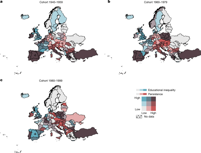
We estimate the degree of intergenerational mobility of education for three cohorts—1940–1959, 1960–1979 and 1980–1999—by regressing the years of education of individuals on those of their highest educated parent, controlling for sex and survey year fixed effects62. The subdivision of the sample into three cohorts enables us to estimate intergenerational educational mobility with a sufficiently large sample size of individuals for each country and region. In the case of missing information for one parent, we use the level of education of the available parent. As years of schooling varies between countries, we use modified ISCED measures to generate a harmonized measure of years of schooling. Using the ESS-ISCED measure, available from wave 5 onward, as the basis, we harmonize observations from earlier waves (Supplementary Tables 13 and 14), and assign an ordinal scale (Supplementary Table 15).
We refer to this indicator of intergenerational mobility as the slope coefficient. However, given potential distributional differences between the two generations, we additionally multiply the slope coefficient with the ratio of s.d. of parents’ and children’s years of education to obtain a measure of standardized persistence. These two measures are non-directional and origin-independent, capturing both upward and downward movements across the entire distribution. In both cases, the higher the indicator, the lower is intergenerational mobility. Both measures are standard in the literature on intergenerational educational mobility and constitute valuable summary indicators for equality of (educational) opportunity63,64. Furthermore, educational mobility measures are strongly correlated with income mobility63. To test the consistency of our estimates, we compared our country-level indicators with those included in the World Bank’s Global Database on Intergenerational Mobility17. Reassuringly, at the cohort-country level, the Pearson correlation coefficient is 0.86 for years of education (P < 0.001; n = 105), and 0.66 for intergenerational mobility (P < 0.001; n = 105).
In our application, a selection of our results using the slope coefficient (persistence) is shown in Table 1, and all specifications are presented in Supplementary Table 5. Those using standardized persistence (Supplementary Table 7) are consistent with the main findings.
Constructing an annualized panel
To link past intergenerational mobility with contemporary economic changes, the cohort-specific mobility indicators and cohort-specific initial conditions are transformed into annual time-series measures whereby the indicator value of a given cohort is weighted by the expected contribution of cohort members to the economy in a given year14. For example, to compute the profile I weights that can be attributed to a given cohort for each year, we use the share of each cohort’s expected effective labour supply over the total effective labour supply in a given year based on per-capita effective labour profiles over the life cycle65. We therefore define the measures obtained using this methodology as indicators of effective mobility. To permit robustness testing of the results from our application, investigating the relationship between mobility and innovation, we also applied four alternative weighting procedures.
For profile II and III weights, we used innovation life-cycle profiles first for all patenting activity and, second, for highly cited patenting activity, respectively66. For profile IV and V weights, we used the Luxembourg Income Study (LIS) database, accessed through LISSY, to construct cohort–year–country contribution profiles for both employment and total individual income. The results are consistent across all weighting schemes. We present results obtained using the effective labour supply weights in the main text, those derived from innovation life-cycle profiles and LIS-derived employment, and income measures are shown in Supplementary Tables 8 and 9 for persistence and standardized persistence, respectively.
The variation across years and regions is given by the interaction between intergenerational mobility and the weight, while, by construction, the methodology used to compute the effective measure of mobility P allows us to test one side of the relationship between intergenerational mobility and innovation while avoiding issues related to reverse causality. Thus, the association between intergenerational mobility and innovation in the estimations is driven by younger cohorts entering the labour market and gaining labour market experience, while older cohorts age and correspondingly reduce their labour force participation14.
The transformation of cohort-specific mobility measures into composite annual measures gives an index, which we define as our measure of effective mobility:
$${P}_{{rt}}=\mathop{\sum }\limits_{c=1}^{C}{w}_{{ct}}{p}_{{cr}}$$
(4)
where the intergenerational persistence index P in region r for each year t is the weighted average mobility of people born in cohort 1940–59 (c = 1), 1960–79 (c = 2) or 1980–99 (c = 3), that is, the sum of the persistence of each cohort (p) multiplied by the respective cohort-participation weight (w). Hereby, the three weights sum up to one for each year.
Supplementary Fig. 1 depicts the age-participation profiles used to apply the aforementioned procedure for profile I–III weights. Using per-capita effective labour profiles over the life cycle as an example, wct is the share of the cohort’s effective labour over the total effective labour supply in a given year.
After computing the relative contribution by age as an integral fraction of the respective participation profile, absolute cohort weights at time t are computed by cohort as a sum of the contribution of the in-range ages in year t (for example, in t = 2007, the oldest members of c = 1 are no longer in range). Relative cohort weights are then computed as the share of the cohort weight in t over the sum of cohort weights in t yielding wct. For profile I–III weights, Supplementary Fig. 2 shows the respective weights for each cohort in every year.
For profile IV and V weights, extractions from the LIS database were used to directly compute relative cohort weights as the share of a given cohort’s contributions to the economy in country n at time t over the sum of all contributions in nt yielding wnct, such that:
$${P}_{{rt}}=\mathop{\sum }\limits_{c=1}^{C}{w}_{{nct}}{p}_{{cr}}$$
(5)
We do this for both relative employment shares (profile IV) and relative total individual income shares (profile V), as depicted in Supplementary Fig. 3. In contrast to profile I–III weights, this permits cross-country variation in the weighting procedure.
Application: empirical strategy
Using the weighted panel measures described previously, we test whether higher levels of intergenerational mobility are associated with innovation at the regional level. To do so, we estimate a linear panel regression based on the time series for each region, including confounders potentially affecting the relationship between the two variables (all covariates are described in Supplementary Table 3; the correlation matrix for the covariates used in our main specification is shown in Supplementary Table 4). For regions encompassed by the former Warsaw Pact countries with the addition of the former Yugoslavia and East Germany, we limit the time series to 1992 onward to account for potential patent data mismeasurement arising from inconsistent reporting to PATSTAT. For all other regions, the time series begins in 1985.
The fully saturated regression specification takes the form:
$${Y}_{{rt}}=\alpha +\delta {P}_{{rt}}+{\theta {\bf{X}}}_{{rt}-1}+\varPsi {{\bf{I}}}_{{rt}}+{\tau }_{t}+{\gamma }_{r}+{\varepsilon }_{{rt}}$$
(6)
where Y is innovation in region r and year t. P is the degree of intergenerational persistence, as a weighted average of the persistence of the three cohorts (as previously described). X is a vector of contemporary controls for region-specific characteristics in t − 1, namely proxy measures for local economic activity extracted from daytime satellite imagery collected via Landsat satellites48. l is a vector of controls for cohort-specific characteristics: average years of education, and the coefficient of variation for years of education, and cohort-specific initial conditions, again as a weighted average across the three cohorts. To reduce dimensionality, the cohort-specific initial conditions are included as a single-index variable, summarizing precipitation, temperature, sea level pressure, relative humidity, wind speed and global radiation using factor analysis. Fixed effects are included for year (\({\tau }_{t}\)) and region (\({\gamma }_{r}\)), and in one specification, we additionally control for country-specific time trends by including country dummies interacted with a linear time trend, instead of time fixed effects. \(\varepsilon \) is the error term.
In this analysis, we define regions r as an augmentation of the NUTS 1 level, taking a three-step hierarchical approach to spatial scale: (1) countries in which the NUTS 0, NUTS 1 and NUTS 2 levels are identical (that is, they comprise the entire country) enter the analysis as entire countries (for example, Cyprus and Montenegro). (2) For countries where the NUTS 0 and NUTS 1 levels are identical (that is, the NUTS 1 but not the NUTS 2 level encompasses the entire country), we use the NUTS 2 definition of regions to define the subnational level (for example, the Czech Republic, Ireland and Switzerland). (3) For all other countries, we use the NUTS 1 subnational level (for example, Germany, Poland and the United Kingdom). The augmented NUTS 1 level therefore represents subnational regions whenever possible. Supplementary Fig. 4c depicts the augmented NUTS 1 level, corresponding to 148 regional units. Supplementary Fig. 9 illustrates the (unweighted) number of observations in the ESS pooled data used to construct the weighted cohort-level estimates of intergenerational educational mobility for the baseline sample at the augmented NUTS 1 level.
For our main analysis, we use the version of the EUROPE-IGM-ATLAS that excludes first-generation migrants. A subset of results obtained using profile I weights for effective labour contributions over the lifecycle are presented in Table 1, examining the relationship between the slope coefficient persistence and innovation captured by the inverse hyperbolic sine transformation of the number of patents. The results with all regression specifications are presented in Supplementary Table 5. In Supplementary Table 6, we alternatively measure innovation using granted patents and citation-weighted patents. In Supplementary Table 7, we alternatively use standardized persistence as our measure of persistence. In Supplementary Tables 8 and 9, we examine the relative robustness of our results to the weighting procedure, using the annualized indices computed based on alternative weighting profiles for persistence and standardized persistence, respectively.
Application: additional considerations
The results of a further series of tests, considering the three different definitions of the dependent variable (patent count, granted patent count, citation-weighted patent count), the two measures of intergenerational persistence (persistence and standardized persistence), the iterative inclusion of covariates (described in Supplementary Table 3) corresponding to seven regression specifications (Supplementary Table 5), the five weighting profiles and using two different samples to construct the cohort-level measures of intergenerational persistence ((1) excluding first-generation migrants only, and (2) additionally excluding individuals with a migration background, respectively), are reported in Extended Data Fig. 3. Extended Data Figure 3a presents the results of this procedure, demonstrating the distribution of 420 estimated coefficients and corresponding elasticities. In Extended Data Fig. 3b, we limit these to our preferred specification only (Table 1 (column 3) and Supplementary Table 5 (column 6), respectively). In Extended Data Fig. 4, we demonstrate how the iterative inclusion of controls affects these estimates.
Furthermore, in Supplementary Table 10, we report estimates for the two alternative versions of the database, for which our indices were computed using different sample restrictions. Supplementary Table 10a presents results for a sample that excludes both first- and second-generation migrants, while Supplementary Table 10b includes both migrants and non-migrants. However, while both are consistent with the baseline analyses, we regard Supplementary Table 10b as the least consistent owing to potential selection biases (given, on one hand, that the education outcomes of first-generation migrants are potentially unaffected by the localized opportunity structure conditional on age-at-migration and, on the other hand, that selective migration to high opportunity and highly innovative areas is probably endogenous).
Next, to investigate to what extent the labour-force contribution weights that we use to construct our annualized measures of persistence contribute to the variation of the regressor, we conduct two analyses. First, we decompose the variation in persistence (P), our main independent variable, in our regression sample according to the law of total variance. The results of this decomposition, presented in Supplementary Table 18, reveal that, across all five weighting profiles, the cohort-specific mobility measure (p) explains a much larger proportion of the total variance in our main independent variable than the contribution weights (w). That is, the variation in the regressor is not primarily driven by the contribution weights. Second, we use procedures from the literature on shift-share instrumental variables67,68 to analyse which components of the regressor contribute to its variation. The results of this analysis, presented in Supplementary Fig. 10, reveal that all cohorts contribute fair shares to the regressor’s variation and that no single cohort or year predominantly drives this variation.
Moreover, as our dependent variables represent fractional counts, as an alternative estimator we consider Poisson pseudo maximum likelihood (PPML) with untransformed independent variables. The PPML estimator is particularly well suited to fractional count dependent variables that include zero values, and also accounts for a multiplicative and heteroskedastic data-generating process, which can occur in patent count data69. However, PPML and other related generalized linear models with log link have been found to be more sensitive to the influence of observations with extreme values70,71,72, which in our data occur due to regional differences in the level of patenting activities. Therefore, the PPML results could differ from our main results if, for example, our main regression does not adequately reflect the data-generating process underlying patent counts, or if a few extreme observations exert large influence.
Replicating our baseline analyses using the PPML estimator, the full set of PPML results in Supplementary Fig. 5 reveals a high but smaller share of statistically significant negative estimates (52%, two-sided Wald tests with P < 0.1), and a non-negligible share of statistically significant positive estimates (24%) compared with those estimated using linear regressions with inverse hyperbolic sine transformed dependent variables (89% statistically significant negative estimates, no significant positive estimates). To test whether this difference in the results originates from few influential observations, we divide our sample into two subsamples based on the distribution of patent count averaged over our observation period at the augmented NUTS 1 regional level, such that every region in our sample is unambiguously assigned to one of the two subsamples. The first subsample comprises regions in the top 10% of the distribution (that is, potentially extreme observations with high influence—or innovation hubs) and the second subsample comprises the remaining regions. Supplementary Fig. 6 shows the elasticities obtained from the subsamples and those obtained with the full sample. Supplementary Fig. 6a reports results from linear estimation using the inverse hyperbolic sine-transformed dependent variables, while Supplementary Fig. 6b presents the corresponding PPML estimates.
The results show that the distribution of PPML estimates in the non-hub sample (90% of the observations) resembles that of the baseline analysis very closely, with a substantially higher share of negative and significant estimates (66%). Notably, innovation hubs behave differently. For innovation hubs, the shares of significant positive estimates are higher than the shares of significant negative estimates (71% versus 6%) while the elasticity distributions are more widespread—a pattern that the linear estimates for this subsample also confirm (57% significant positive estimates versus 20% significant negative estimates). These differences in the results between the two subsamples support the explanation that the overall differences between our main results and the PPML results stem from few observations exerting a high degree of influence. Overall, the results support the conclusion that intergenerational educational mobility is positively associated with innovation across most regions in our sample, while major innovation hubs constitute an important exception. We discuss potential explanations for this phenomenon in the main text.
Finally, drawing on the suggestive evidence in Fig. 3 as motivation, we examine potential nonlinearities in the relationship between intergenerational mobility and innovation by allowing persistence to enter the analysis in a flexible, nonparametric way. We estimate variants of our preferred specification and compute predicted outcomes across flexible bins of the independent variable, retaining the full set of covariates as well as year and region fixed effects. Supplementary Figs. 7 and 8 present the resulting patterns separately for the three dependent variables (patent count, granted patent count and citation-weighted patent count) and for both linear and PPML estimation. The estimates confirm the qualitative patterns of the baseline analysis: marginal returns to intergenerational mobility increase at medium and high levels of persistence, but flatten or slightly decline when persistence is low (that is, when intergenerational educational mobility is already saturated).
Database structure
The EUROPE-IGM-ATLAS database that we constructed in this study encompasses 36 European countries, 108 mesoregions (NUTS 1) and 225 microregions (NUTS 2), with measures available at several spatial scales. To ensure cross-national and cross-temporal comparability, all regional units in the EUROPE-IGM-ATLAS are harmonized to consistent NUTS-based spatial definitions following the procedure described in the ‘Materials’ section. The harmonized regional classification is primarily based on the 2016 NUTS framework, with the exception of Poland, for which the 2008 NUTS boundaries are retained owing to later regional redefinitions.
Indices are available for (1) two measures of intergenerational mobility, persistence (as measured by the slope coefficient) and standardized persistence (the slope coefficient multiplied by the ratio of s.d. of the parents’ and children’s years of education); (2) educational inequality (as measured by the coefficient of variation) for both parents and children; and (3) average years of education for both parents and children. In the cohort-level version of the database, we also include information on the weighted and unweighted number of observations used in the indices’ construction for each region–cohort pair.
The database is currently available both cohort-wise and in annualized weighted form, with each of the aforementioned weighting schemes applied. Annualized weighted measures are available 1985–2025, with the exception of profile IV and V weights, which are currently available until 2023 given the availability of data extracted from the LIS used to construct the weights. Finally, both the cohort-linked measures and the annualized weighted measures are available in three versions, based on the samples used in the indices’ construction: (1) excluding first-generation migrants only; (2) excluding all individuals with a migration background; and (3) including all migrants. See Supplementary Table 11 for clarification on versioning.
Ethics statement
This study exclusively uses publicly available secondary data sources that do not contain personally identifiable information. No human participants were directly involved in the research, and no individual-level data were collected by the authors. Accordingly, the study was exempt from institutional review board and ethics committee approval.
Reporting summary
Further information on research design is available in the Nature Portfolio Reporting Summary linked to this article.

