


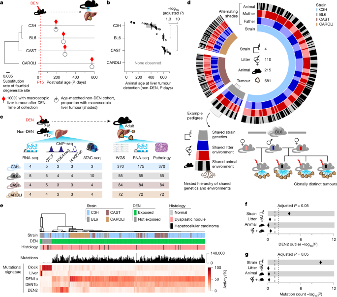
The key reagents and resources required to replicate our study are listed in Supplementary Table 2.
Mouse colony management
Animal experimentation was carried out in accordance with the Animals (Scientific Procedures) Act 1986 (UK) and with the approval of the Cancer Research UK Cambridge Institute Animal Welfare and Ethical Review Body: the maximum approved tumour burden was 10% body weight, which was not exceeded. Animals were maintained using standard husbandry: mice were group-housed in Tecniplast GM500 IVC cages with a 12 h–12 h light–dark cycle (07:00–19:00) and ad libitum access to water, food (LabDiet 5058) and environmental enrichments.
The following mouse strains and species were used: M. musculus domesticus C3H/HeOuJ (C3H mice) and C57BL/6J (BL6), M. musculus castaneus CAST/EiJ (CAST) and M. caroli CAROLI/EiJ (CAROLI; Supplementary Table 2). For simplicity, these strains, subspecies and species are here referred to as ‘strains’.
Chemical model of hepatocarcinogenesis
We treated 15-day-old (P15) male mice of all strains with a single intraperitoneal injection of DEN (N0258, Sigma-Aldrich; 20 mg kg−1 body weight) diluted in 0.85% saline. This is a well-established tumour-induction protocol and therefore DEN treatment was not randomized or blinded. Injections were performed in a fixed-time interval between 08:00 and 09:00 to control for circadian effects in DEN metabolism. Liver tumour samples were collected from DEN-treated mice 25 weeks (C3H), 36 weeks (BL6), 38 weeks (CAST) or 78 weeks (CAROLI) after treatment; pilot data indicated that 100% of surviving DEN-treated mice would develop tumours by these timepoints. The time of tumour removal was recorded for DEN-exposed BL6 mice, with 5-min intervals added for each sequential tumour isolated (Extended Data Fig. 9a–e). Our existing cohort of 370 C3H tumours25 included multiple tumours per animal and multiple animals per litter. To capture this hierarchical structure across genetic backgrounds, we included a minimum of 50 tumours per strain.
Untreated control mice from each strain were assessed for the presence or absence of tumours at the same ages as DEN-induced tumours to assess inherent susceptibility to spontaneous tumours (Fig. 1a and Supplementary Table 3). In addition, spontaneous liver tumours were collected from untreated mice identified opportunistically as part of routine colony health surveillance (including one female mouse; Fig. 1b and Supplementary Table 3). All macroscopically identified tumours were isolated and processed in parallel for DNA and RNA extraction and histopathological examination. Additional tissues from untreated P15 mice (ear, tail and liver), untreated age-matched adult mice (liver only; C3H 27 weeks, BL6 38 weeks, CAST 40 weeks and CAROLI 80 weeks) and DEN-treated background (non-tumour) liver (BL6 38 weeks) were sampled for control experiments.
Tissue collection and processing
Liver tumours of sufficient size (2 mm or larger diameter) were bisected; one-half was flash frozen in liquid nitrogen and stored at −80 °C for DNA and RNA isolation, and the other half was processed for histology. Tissue samples for histology were fixed in 10% neutral-buffered formalin for 24 h, transferred to 70% ethanol, machine processed (Leica ASP300 Tissue Processo) and paraffin embedded. All formalin-fixed paraffin-embedded sections were 3 μm in thickness.
Histochemical staining
Formalin-fixed paraffin-embedded tissue sections were stained with haematoxylin and eosin (H&E) using standard laboratory techniques. Histochemical staining was performed using the automated Leica ST5020; mounting was performed on the Leica CV5030.
Whole-slide image acquisition
Tissue sections were digitized using the Aperio XT system (Leica Biosystems) at 20× resolution; all H&E images are available in the BioStudies archive at EMBL-EBI under accession numbers S-BSST383 (ref. 25) and S-BSST384 (this study).
Tumour histopathology
H&E sections of liver tumours were blinded and assessed twice by a histopathologist (S.J.A.). Tumours were classified as dysplastic nodule or hepatocellular carcinoma (HCC) according to the International Harmonization of Nomenclature and Diagnostic Criteria for Lesions in Rats and Mice guidelines55. In addition, tumour grade, size, morphological subtype, nature of steatosis and mitotic index were assessed (Supplementary Table 1), as well as the presence of cystic change, haemorrhage, necrosis or vascular invasion.
Sample selection for computational pathology, WGS and RNA-seq
Tumours that met the following histological criteria were selected for WGS (n = 370 for C3H, n = 55 for BL6, n = 84 for CAST and n = 72 for CAROLI): (1) diagnosis of dysplastic nodule, (2) homogenous tumour morphology, (3) tumour cell percentage of more than 70%, and (4) adequate tissue for DNA and/or RNA extraction. Neoplasms with extensive necrosis, mixed tumour types, a nodule-in-nodule appearance (indicative of a HCC arising within a dysplastic nodule) or contamination by normal liver tissue were excluded. As carcinogen-induced tumours arising in the same liver are independent24, multiple tumours were selected from each mouse to minimize the number of animals used. A subset of normal (non-tumour) samples from untreated age-matched mice were also whole-genome sequenced (n = 13 for C3H, n = 11 for BL6, n = 7 for CAST and n = 14 for CAROLI). In addition, a small number of HCC tumours were subject to WGS and released in the accompanying data, but were excluded from the analyses reported in this article (n = 1 for C3H, n = 11 for BL6, n = 0 for CAST and n = 4 for CAROLI).
Computational pathology analysis
Whole-slide images (WSIs) of tumours were annotated in QuPath (v0.2.2)56 using the polygon tool to include neoplastic tissue and exclude adjacent parenchyma, cyst cavities, processing artefacts and white space. For tumours with multiple transections, only a single WSI was used. Annotations were reviewed for quality by two histopathologists (S.J.A. and J.C.). Annotated regions were tessellated into fixed size, non-overlapping 256 µm × 256 µm tiles using Groovy in QuPath. For segmentation of epithelioid nuclei, a pre-trained StarDist57 model (he_heavy_augment.zip) was downloaded (https://github.com/stardist/stardist-imagej/tree/master/src/main/resources/models/2D) and an inference instance was deployed using Groovy across the tiles in QuPath, built from source with Tensorflow58, with a minimum detection threshold of 0.5. Quantitative geometric features (size and shape) were measured for each nuclear object (Supplementary Table 1). The object-level measurements were subsequently abstracted by computing the median, standard deviation, interquartile range and kurtosis for each tile and WSI. Nuclear volume was subsequently calculated using the median nuclear diameter per slide.
Digitized histology images of DEN-induced tumours are available from Biostudies: accession numbers S-BSST383 (ref. 25) and S-BSST384 (this study).
DNA and RNA isolation
Simultaneous isolation and purification of genomic DNA and total RNA from tumours, background DEN-exposed liver tissue and untreated normal liver tissue was performed using AllPrep 96 DNA/RNA kit (80311, Qiagen) according to the manufacturer’s instructions. DNA from P15 liver tissues was isolated and purified using the AllPrep DNA/RNA mini kit (80204, Qiagen); total RNA was extracted using QIAzol Lysis Reagent (79306, Qiagen) according to the manufacturer’s instructions. Genomic DNA was isolated from ear or tail samples using the DNeasy blood and tissue kit (69504, Qiagen) according to the manufacturer’s instructions.
WGS
Genomic DNA quality was assessed on a 1% agarose gel and quantified using the Quant-IT dsDNA Broad Range Kit (Q33130, Thermo Fisher Scientific). Genomic DNA was sheared using a Covaris LE220 focused-ultrasonicator to a 450-bp mean insert size.
WGS libraries were generated from 1 μg of 50 ng µl−1 high-molecular-weight genomic DNA with a Saccharomyces cerevisiae spike-in control (1 ng of 900 pg µl−1 genomic DNA; 69240, Merck Millipore) using the TruSeq PCR-free Library Prep Kit (20015963, Illumina) according to the manufacturer’s instructions. Library fragment size was determined using a Caliper GX Touch with a HT DNA 1k/12K/Hi Sensitivity LabChip and HT DNA Hi Sensitivity Reagent Kit to ensure 300–800 bp (target of approximately 450 bp).
Libraries were quantified by real-time PCR using the Kapa library quantification kit (KK4824, Kapa Biosystems) on a Roche LightCycler 480. We pooled 0.75 nM libraries in six-plex and sequenced them on a HiSeq X Ten (Illumina) to produce paired-end 150-bp reads. Each pool of six libraries was sequenced over eight lanes (minimum of 40× coverage).
WGS FASTQ files are available in the European Nucleotide Archive at EMBL-EBI under accession PRJEB37808 (ref. 25) and PRJEB15138 (this study).
WGS read alignment
Alignment of WGS data was performed as previously described25. In brief, sequencing reads were aligned to their respective genome assemblies from Ensembl (v.91)59, (BL6 = GRCm38 = GenBank: GCF_000001635.26, C3H = C3H_HeJ_v1 = GenBank: GCA_001632575.1, CAST = CAST_EiJ_v1 = GenBank: GCA_001624445.1, CAROLI = CAROLI_EiJ_v1.1 = GenBank: GCF_900094665.2) using bwa-mem (v0.7.12)60. The yeast reference genome S228c (GenBank: GCA_902192305.1) was included in the alignment targets to account for the spike-in DNA. Using WGS of non-tumour liver, ear and tail samples (described above) collected and sequenced contemporaneously with tumour samples, regions of abnormal WGS read coverage were identified25 and subsequently masked from the analysis (percentage of the reference genome masked: BL6 = 5.5%, C3H = 12.7%, CAST = 11.5% and CAROLI = 12.5%).
Variant calling and mutation filtering
Single-base substitution (SBS) mutations were called using Strelka2 (v2.8.4)61. As described in ref. 25, fixed genetic differences and segregating germline variants within our colonies were identified and discarded. Indel mutations were filtered with identical parameters to SBS mutations with the additional criteria that (1) each called indel mutation must be supported by at least three independent reads, and (2) where the same indel mutation was found in at least two tumours from the same animal and shared between more than 50% of tumours from that animal, it was filtered from the calls of all tumours within the strain. This latter ‘animal-level-filtering’ step removes fixed and segregating germline indels that passed the familial clustering filter due to the conservative calling of indels relative to SBS mutations. Of the 4,446 indel mutations subject to animal-level filtering (distinct sites, not summing repeat occurrences over tumours), only two are predicted by Variant Effect Predictor (VEP; v109.3)62 to disrupt protein sequence (genes Atxn2l and Cyp4a30b).
Mutational rate calculations
For lesion-strand resolved analyses, SBS mutational rates were calculated as 192 category vectors representing every possible single-nucleotide substitution conditioned on the identity of the upstream and downstream nucleotides. Each rate being the observed count of a mutation category divided by the count of the trinucleotide context in the analysed sequence. For lesion-strand non-resolved analyses, the same procedure was followed but reverse complement mutation (for example, T→C and A→G) and sequence context (for example, ATG and CAT) counts were combined to give 96 category vectors, which by convention are presented oriented as a mutation from the pyrimidine base of the base pair. Indel rates were calculated as indel count per megabase, per tumour and corrected for the expected diploidy of autosomes.
Mutational signature analysis
SBS mutational signatures were defined and deconvolved using the R NMF library (v0.28) nmf function63 with rank = 5, run =1,500 and the method set to use the Brunet algorithm64. The rank defines the number of signatures to identify; the value of 5 was selected after testing ranks 2 to 8 inclusive and selecting the first value of rank for which the cophenetic coefficient substantially decreases64. This value also coincided with an inflection point in the curve plotting the residual sum of squares against rank, as proposed as an alternate method for optimal rank choice65.
Indel mutational signatures were generated using SigProfiler (v1.2.19)66 using the corresponding strain-specific reference assemblies (masked, see above). Bootstrap replicate datasets were generated using the SigProfilerMatrixGenerator for the calculation of 95% confidence intervals. For the analysis of multi-nucleotide indel sequence composition, only tumours with cellularity estimated at more than 50% were considered and indels of length greater than 1 bp were folded into unique discrete sequence categories combining repeat unit repetition and reverse-complement relationships, for example, AC deletion encompasses AC, CA, GT and TG deletion. Insertions and deletions were categorized by length (span of deleted or inserted nucleotides) and the mutational rates for each sequence category (for example, AC) calculated as the number of events (for example, AC deletions) divided by the number of that sequence context in the reference genome (for example, AC occurrences). Percentage rates were calculated (for example, AC deletion rate as a percent of the sum of dinucleotide category deletion rates) and compared between strains (Extended Data Fig. 1o–q); the comparison of rates thus controls for the minor sequence composition differences between the genomes of the four strains. The 95% confidence intervals were obtained from 100 bootstrap samples of the tumours for analysis within each strain.
Mutational asymmetry segmentation and scoring
The lesion segregation model predicts that whole chromosomes would be coherently strand asymmetric for mutations following a burst of DNA damage. Although this is often the case, homologous repair in the first round of DNA replication following damage can result in sister chromatid exchange (SCE) events and discrete transitions in the mutational asymmetry of the chromosome such that chromosomes are made up of multi-megabase blocks of alternating mutation asymmetry25,26. We refer to these blocks as genomic segments. Genomic segmentation on mutational asymmetry was performed as previously reported25. Mutational strand asymmetry was scored for each genomic segment using the relative difference metric S = (RT − RA)/(RT + RA) where RT is the rate of mutations from T on the forward (plus) strand of the reference genome and RA is the rate of mutations from A on the plus strand, equivalent to the rate of mutations from T on the reverse (minus) strand.
Identifying and filtering reference genome mis-assemblies
Mutational asymmetry patterns arising from lesion segregation allow the long-range phasing of chromosome strands, which can be used to detect discrepancies in sequence order and orientation between the sequenced genomes and the reference. We identified autosomal asymmetry segments that immediately transitioned from forward strand bias (S > 0.33) to reverse strand (S < −0.33) or vice versa without occupying the intermediate unbiased state (−0.33 ≥ S ≤ 0.33); such discordant segments are unexpected. Allowing for ±100-kb uncertainty in the position of each exchange site, we produced the discordant segment coverage metric. At sites with discordant segment coverage of more than 1, we calculated relative enrichment for misassembly M = (ds − cs)/(ds+cs) where ds is the number of discordant segments over the exchange site and cs the number of concordant: where either forward or reverse mutational asymmetry extends at least 1 × 10⁶ nucleotides on both sides of the exchange site. Values of M > 0 indicate consensus for misassembly. The approximate genomic coordinates for a C3H strain-specific inversion on chromosome 6 have been previously reported67.
Classification of mutational asymmetry
On the basis of previously described mutational asymmetry segmentation and scoring, samples were classified based on their adherence to the expectations of lesion segregation, that is, asymmetric or non-asymmetric25. First, to reduce noise and minimize the influence of large copy number alterations (CNAs) and aneuploidies, genomic segments with fewer than 100 mutations and those with significantly higher or lower than average read depth were removed (P < 0.05, probability of each segment being sampled from a normal distribution with mean and standard deviation equal to the weighted mean and standard deviation of the per-segment means). Genomic segments were classified as symmetric (abs(S) < 0.2, where abs(S) is the absolute value of the previously defined mutational asymmetry parameter S), asymmetric (abs(S) > 0.8) or intermediate (abs(S) ≥ 0.2 and ≤0.8). For each tumour, the proportion of the genome belonging to each class was calculated. Samples with less than 10% asymmetric autosomes were defined as non-asymmetric (symmetric). All remaining samples were classified as asymmetric. As SCE events can be identified only in the presence of mutation asymmetry, the non-asymmetric tumours were excluded from SCE rate calculations.
Tumour cellularity estimates
As described in ref. 25, variant allele frequency (VAF) was calculated as (1 − R/d), where R is the reference read count at a mutated site and d is the total read depth at the site. For each tumour, the modal VAF was determined using the function ‘amps’ from the R package modes (0.7.0) to detect the size and position of the largest peak in the VAF density distribution. Cellularity was then calculated as ploidy × the major peak VAF, in which ploidy was set as 2 for all samples, except CAROLI tumours with no mutational asymmetry, which were inferred to be whole-genome duplicated (ploidy = 4).
Large copy number variant calling
Tumour genomes were segmented on the basis of their change in read depth, relative to untreated adult liver samples (n = 11 for BL6, n = 11 for C3H, n = 14 for CAROLI and n = 7 for CAST) using CNVkit (v0.9.6)68. To suppress calling of small CNAs, minimum segment size was set as 1 Mb. For each segment, copy number (CN) was calculated using the log2 read depth fold change (FC) given by CNVkit, and the sample ploidy (p) and cellularity (c), where: CN = ((2FC − 1 + c)/c) × p. Within strain, CN estimates were adjusted for read depth biases by subtracting the median change in CN of all overlapping segments (overlapping defined as segments where the intersect is 80% or more of the union, adjustment performed for segments with 3 or more overlapping segments, change in CN calculated as CN − p). Segments with adjusted CN within 0.15 of the sample ploidy were discarded. Segments with adjusted CN within 0.15 an integer were called as clonal CNAs. Segments outside this threshold were identified as subclonal CNAs. Filtering was then performed to remove recurrent artefactual CNAs by discarding any short CNA (less than 10% of total chromosomal length) with 80% or more overlap of another CNA from the same strain.
Aneuploidies were identified as either gain or loss of chromosomal segments totalling more than 80% of a chromosome; typically these were whole-chromosome (100%) gains and losses. Significant recurrence was identified by randomly permuting aneuploidy labels across autosomes. P values were calculated by comparing the observed recurrence of a specific aneuploidy to the null distribution of random recurrence generated by 10,000 permutations. Aneuploidies with P < 0.05 Bonferroni-corrected significance were identified as having significant recurrence.
Telomere length analysis
Two complementary approaches were used for telomere length analysis. First, telomerecat (v4.0.1)69 was applied using default settings to whole-genome-sequenced samples aligned to the strain-matched reference genome (see above). The telomere length metric was estimated for each sample, which attempts to take into account ploidy changes, other changes in telomere count and interstitial (non-telomeric) telomere repeats in the reference genome. However, the quality of genome assembly systematically differs between the four strains in this study so a second, reference alignment free, approach was used to allow direct comparison between strains without confounding assembly differences. Using samtools view (v1.9)70 and Unix shell scripting (grep), WGS reads were identified that contained three perfect consecutive matches to the telomeric repeat sequence (TTAGGG)3 or its reverse complement (CCCTAA)3. All instances of the single TTAGGG or CCCTAA repeat were counted in, and summed over, those reads. The raw counts of telomere repeats were normalized to 1× haploid genome coverage using read alignment to the reference genome. Telomerecat and grep-based estimates of telomere length were highly correlated (Spearman’s ρ = 0.616, P = 1.54 × 10−64), but a small number of extreme discrepancies were identified that represented either zero-length or implausibly large telomeres reported by telomerecat. For these reasons, and the fair direct comparison between strains, the main results are reported using the grep-based method, but qualitatively, the same conclusions can be drawn from the telomerecat-based analysis.
Multiallelic mutational rates
Aligned reads spanning genomic positions of somatic mutations were re-genotyped using samtools mpileup (v1.9)70. Genotypes supported by two or more reads with a nucleotide quality score of 20 or more were reported, considering sites with two alleles as biallelic, those with three or four alleles as multiallelic. To simplify analysis and interpretation, multiallelic rates were calculated only for mutations from A or T nucleotides (C and G lesions contribute to both DEN1 and DEN2 signatures and have differing propensities for multiallelic variation, and the signatures vary in their contributions between tumours). The multiallelic rate is the fraction of mutations from A or T in a tumour that are identified as multiallelic in that tumour. The multiallelic rate was calculated (1) as an average for each tumour, and (2) separately for each mutation asymmetry segment of each tumour.
MRCA generation
Following previous work, we estimated cell generation post-mutagenesis of the MRCA of the cells in the sequenced tumour based on the fraction of autosomal genomic segments that are multiallelic25. Genomic segments were defined per tumour using mutational asymmetry, as described above. After the first cell division post-damage, each segment will contain two lesion-containing strands, which will be diluted through subsequent divisions. The scenarios where one or both lesion strands of a segment are multiallelic are not readily distinguishable from the data, as in both cases the segment will appear as multiallelic. However, the fraction of non-multiallelic segments, where both lesion strands are lost, is directly observable from the data. We called a segment non-multiallelic if less than 4% of mutated sites are multiallelic. Let p be the fraction of autosomal lesion containing strands, and q = 1 − p. Assuming independent segregation of DNA copies per segment, the expected fraction of autosomal segments without multiallelism (MA) is q2, and thus we estimate p as 1 − (fraction of segments without MA)½.
Tumours with more than 75% or 0% of segments showing multiallelism were assigned generation 1 and generation ≥5 MRCAs, respectively. For the remaining tumours, we estimated the MRCA generation using maximum likelihood under the following rationale. At generation 1 post-mutagenesis, we expect 100% of segment copies to have a lesion-containing strand and thus show multiallelism. At each subsequent generation, a segment loses one of its lesion-containing strands, and thus its ability to generate multiallelism with probability 0.5: hence, the probability of retaining an individual lesion strand at generation n post-mutagenesis is 2(−n + 1). With independent segregation, the probability of no lesion strands in a segment at generation n is thus (1 − 2(−n + 1))2. In a tumour with x autosomal segments, assuming segment independence, the observed segment number without multiallelism is thus distributed as binomial (x, (1 − 2(−n + 1))2). Ranging over n = 2, 3, 4, 5, we selected the n value that maximizes the likelihood of the observed data under this binomial model, resulting in an inference of the MRCA generation of the tumour.
Uniformity of post-MRCA growth
To quantify the balanced:unbalanced contribution of lineages post-MRCA (uniformity of clonal growth), we first identified genomic segments where the two allelic copies of a chromosome have opposite mutational asymmetries, resulting in the segment as a whole being mutationally symmetric (−0.5 ≤ S ≤ 0.5; more conservative asymmetry threshold used based on simulated data). In these mutationally symmetric regions, T→N mutations relative to the reference genome forward strand represent mutations from one lesion strand and A→N mutations represent the other lesion strand of the segment. Calculating multiallelic rates separately for T→N and A→N allows determination of the multiallelic rate resulting from each lesion strand of a segment. Under the rationale that unbalanced lineage contributions would result in higher variation in multiallelic rate (Fig. 5a), within these segments, we further split mutations into non-overlapping windows of 100 neighbouring T→N or A→N mutations, which allowed us to test for balanced retention of lineages within individual tumours. Our test requires only a single assumption, which is that the probability that a mutated site is multiallelic is constant across all sites. Under this assumption and balanced lineage retention, among segments that display multiallelism, the number of multiallelic mutant sites per window follows a truncated binomial distribution, TruncBinom(n, p, a), where n = 100, p is the probability of multiallelism per mutated site, and a is the threshold for a window to be deemed to have non-zero multiallelism (four or more multiallelic sites). Deviations from this distribution indicate non-uniform lineage retention. To test for non-uniform lineage retention, we calculated the overdispersion of the observed windowed multiallelic rates: the variance of these rates divided by the variance expected under the maximum-likelihood best-fitting truncated binomial distribution. Only windows within mutationally symmetric regions and with multiallelic rate ≥ 4% were considered.
To assess the power of this method and its robustness to SCEs, we performed a simulation study. We simulated DEN-induced tumours with generation 1, 2 and 3 MRCAs, and with different numbers of SCEs. We considered both SCEs that occurred at generation 0, which are detectable with mutational asymmetry segment calling, and SCEs that occurred after the first mitotic division, which are undetectable via asymmetry and henceforth termed ‘cryptic SCEs’. We simulated non-uniform lineage retention via selection by varying F, the proportion of the final tumour contributed by the clonally dominant daughter cell of the MRCA from 0.5 (neutral evolution) to 0.9 (highly biased lineage retention). Tumours were simulated for seven generations after transformation, with retained damage generating mutations at each round of replication, according to mutational probabilities matching the observed DEN mutations. We set the probability of correctly incorporating the reference base opposite damage in a single replication to be 0.75, which best matched the typical observed multiallelic rates in our data. We then simulated sequencing at 30× coverage, and applied the same pipeline of calling multiallelic and performing segment calling to the simulated data as to the mouse data. For each simulated tumour, we calculated the overdispersion, and used Monte Carlo simulation of the overdispersion from the best-fitting truncated binomial distribution to test for non-uniform lineage retention (10,000 Monte Carlo simulations per tumour).
In simulations, we observed that cryptic SCEs could potentially inflate our false-positive rate by acting as an alternative, non-uniform mechanism to increase the variance in multiallelic rates. Therefore, we performed a stringent filtering of windows to remove any windows that potentially overlapped a cryptic SCE site, identifying as candidates windows with non-zero multiallelic rate (4% or more) that occurred next to one or more windows with zero multiallelic rate (less than 4%). As this strategy does not account for cryptic SCEs where the breakpoint occurs on the first or last window of a segment, we also removed the first and last window of each type from each segment in our filtering (which resolved this issue in our simulations). The multiallelic overdispersion was calculated for n = 389 tumours, including tumours with inferred generation 1, 2 or 3 MRCAs and that had at least two windows that satisfied the lesion-strand-filtering conditions. For each of these tumours, we then performed Monte Carlo simulations, simulating 1 million draws from the best-fit uniform-growth distribution to each tumour, calculating a P value of our observed overdispersion, which we then Bonferroni corrected, and used to test the null hypothesis, at 0.05 significance, that the tumour grew with uniform retention of lineages. We also note, from simulations, that the value of this overdispersion statistic provides an indication of the extent of biased lineage retention that takes place (Extended Data Fig. 10b).
Genomic annotation
Genic annotation was obtained from Ensembl (v91)59 for the corresponding C3H, BL6, CAST and CAROLI reference genome assemblies (C3H_HeJ_v1, GRCm38, CAST_EiJ_v1 and CAROLI_EiJ_v1.1, respectively). Genomic repeat elements were annotated using RepeatMasker (v20170127)71 with the default parameters and libraries for mouse annotation. Genomic coordinates were transformed between reference genomes using the HAL toolkit (v2.3)72, utilizing the UCSC mouseStrains_1509.hal multi-strain alignment with CAROLI_EiJ_v1.1 added using progressiveCactus (v1.0.0)73. The functional consequences of mutations (for example, amino acid change, splice site disruption and synonymous sequence change) were annotated using Ensembl VEP (v109.3) run in the ensemblorg/ensembl-vep docker container under Singularity; the Ensembl v91 annotation was used for the corresponding reference genome assembly. Phylogenetic distances between strains were calculated using fourfold degenerate (4D) sites, extracted from the HAL alignments using the HAL toolkit hal4dExtract function. 4D site rate calculations were performed using PHAST (v1.3)74 phyloFit under the REV model.
Extrapolating from substitution rates at codon 4D sites (Fig. 1a), there are expected to be 7.5 × 10⁶ single-nucleotide differences genome wide between C3H and BL6. Between BL6 and CAST, 2.5 × 10⁷ single-nucleotide differences are expected. For comparison, between any two randomly selected humans, there are expected to be between 6.4 × 10⁶ and 2.5 × 10⁷ single-nucleotide differences33, placing most human comparisons between BL6:C3H and BL6:CAST in the number of genetic differences.
Driver discovery methods
Protein-coding cancer driver genes were analysed using three computational methods: OncodriveFML (v2.2.0)75, which identifies genes with a bias towards high impacting mutations, OncodriveCLUSTL (v1.1.3)76, which identifies genes containing mutations that are linearly clustered in nucleotide sequence, and dNdScv (v0.1.0)77, which uses a maximum-likelihood approach to quantify selection by identifying genes with an excess of nonsynonymous, essential splice site or truncating mutations.
To increase the sample size, a single pan-strain analysis was performed using all DEN-treated dysplastic nodules (n = 581). Only single-nucleotide mutations that mapped to all four genomes were kept (n = 32,894,997, HAL alignments above). For the OncodriveFML and OncodriveCLUSTL analyses, mm10 was used as the reference genome. The dNdScv analysis was carried out four times; in each iteration, mutations were projected onto the gene annotations of one of the four mouse strains.
To run OncodriveFML and OncodriveCLUSTL, protein-coding sequences from all transcripts in protein-coding genes were merged together into their corresponding gene using pybedtools (v0.8.0)78.
OncodriveFML variant pathogenicity was assessed using GRCm38/mm10 SIFT scores (v83)79. OncodriveFML was run on the pan-strain dataset using strain-specific coding DNA sequence (CDS) normalized trinucleotide background models. These mixed background models allow the method to account for strain-specific differences in the trinucleotide mutational probabilities. These models were computed using bgsignature (v0.2; https://pypi.org/project/bgsignature/). All other OncodriveFML parameters were kept as default. Genes with q < 0.1 were considered candidate drivers.
OncodriveCLUSTL was run using a strain-specific CDS normalized trinucleotide background model, as for OncodriveFML. To improve the accuracy of clustering signals detected in CDS regions, simulated mutations were randomly sampled within coding sequences (simulation mode ‘region_restricted’). Clusters were analysed by concatenating all subsequent CDS regions of a gene. All other parameters were kept as default. Genes with q < 0.01 bearing more than 15 mutations were considered candidate drivers.
To run dNdScv, genome references were built using the GTF (Ensembl v91) annotations of the respective mouse strain. dNdScv was run with the parameters ‘cv = NULL’ and ‘max_muts_per_gene_per_sample = 50’ and genes with q < 0.1 were identified.
Driver event annotation and combinatorial analysis
Candidate driver events including point mutations, protein-coding sequence disrupting indels, WGD and recurrent aneuploidies were encoded as binary variables (either present or absent) for each tumour. For nucleotide substitution and indel mutations any ‘moderate’ or ‘high’ impact mutation annotation in an identified driver gene was considered to be a candidate driver mutation. Where VAF filtering of driver mutations was applied, a tumour was considered to have a driver mutation if the VAF of that mutation exceeded (c/2)/p, where c is the cellularity estimate of the tumour and p is the expected ploidy of the driver locus (autosomal = 2, X chromosome = 1, double those values in WGD tumours).
Evolutionary dependency (co-occurrence and mutual exclusivity) was scored using SELECT (v1.6)80 with default parameters. The wMI P value was used for colour-coding significance and false discovery rate < 0.1 used as multi-testing corrected threshold of significance38. Comparison of driver mutation proportions between strains were performed using the χ2 test implemented in the built-in chisq.test function of R, based on contingency tables of mutation counts.
RNA-seq
Tumour RNA was isolated and purified as described above. RNA concentration was measured using a NanoDrop spectrophotometer (Thermo Fisher); RNA integrity was assessed on a Total RNA Nano Chip Bioanalyzer (Agilent).
Total RNA (1 μg) was used to generate sequencing libraries using the TruSeq Stranded Total RNA Library Prep Kit with Ribo-Zero Gold (20020596 and 20020599, Illumina), according to manufacturer’s instructions. Library fragment size was determined using a 2100 Bioanalyzer (Agilent). Libraries were quantified by quantitative PCR (Kapa Biosystems). Pooled libraries were sequenced on a HiSeq4000 to produce 40 million or more paired-end 150-bp reads per library.
RNA-seq data processing and analysis
Transcript abundances were quantified with Kallisto (v0.43.1)81 (using the flag–bias) and a transcriptome index for each strain compiled from coding and non-coding cDNA sequences defined in Ensembl (v91)59. Expression patterns among the four strains were identified through PCA by combining unnormalized counts for protein-coding genes with orthologues in GRCm38 (Fig. 4a), and per strain from all annotated protein-coding genes and long intergenic non-coding RNAs (Extended Data Fig. 7e,f). The 500 most variable genes were selected in both cases. Transcripts per million estimates were generated for each annotated transcript and summed across alternate transcripts of the same gene for gene-level analysis. Transcription start sites for each gene were annotated with Ensembl (v91) and based on the most abundantly expressed transcript.
RNA-seq data are available at ArrayExpress at EMBL-EBI under accession E-MTAB-8518 (ref. 25) and E-MTAB-16391 (this study).
Differential gene expression analysis
Differential expression was called using DESeq2 (ref. 82) at the gene level after importing estimated counts per transcript from Kallisto using tximport83. Calling was restricted to protein-coding genes and long intergenic non-coding RNAs. Pairwise comparison of differentially expressed genes across strains was performed on the intersection of significantly differentially expressed genes from per-strain dysplastic nodule versus adult normal comparisons (adjusted P ≤ 0.005) after mapping strain-specific IDs to GRCm38 (Extended Data Fig. 7e,f).
Independent component analysis of gene expression
Independent component analysis (ICA) was performed using BIODICA (v0.9)84. The optimal number of components was chosen by BIODICA based on n = 100 iterations of ICA. ICA was applied separately to DEN-induced tumours and to normal (non-tumour) liver samples; for both datasets, expression counts were subject to variance stabilizing transformation before ICA clustering. The Bioconductor package clusterProfiler (v4.14.0)85 was used to identify Gene Ontology and Kyoto Encyclopedia of Genes and Genomes (KEGG) terms over-represented in the high-contribution (key) genes, defined as at least 3 standard deviations from the mean ICA contribution of all genes. For each independent component, we used the annotation with the greatest degree of enrichment (ratio of the number of key genes with the annotation to the number of all genes with the annotation) that had more than five key genes with that annotation and significant term enrichment (Benjamini–Hochberg adjusted P < 0.05).
Enrichment of independent component signatures was evaluated through multinomial log-linear modelling using the R package nnet (v7.3) function multinom with the brglmFit model from the R package brglm2 (v0.9.2). Models were specified including independent component latent factor enrichment and strain identifier. Signatures IC6, IC7 and IC17 were redundant as they closely correlated with strain so were specifically excluded from the model. A MAPK pathway driver gene (or specific mutation for Hras analysis) was defined as the response variable and odds ratios calculated relative to a reference driver (Braf for gene analysis and HrasQ61K for Hras analysis). Statistical tests were Bonferroni corrected for 42 tests in the driver gene-based comparisons and 28 tests in the Hras analysis.
MAPK pathway gene expression analysis
Seventy genes in the MAPK pathway (KEGG pathway: mmu04010 (ref. 86)) were found to be differentially expressed in all strains in a Braf-driven tumour versus adult, age-matched normal liver tissue comparison. Fold changes of these genes, where significant, in Hras-driven and Egfr-driven tumours was consistent with those in Braf-driven tumours (Fig. 4b). Differential expression was called as above, with restriction to tumours with identified driver genes. The expression of the 70 MAPK genes in the combined four-strains dataset described above were used in PCAs (Extended Data Fig. 7g).
Expected mutational rate modelling
To model the expected rate (mutations per million nucleotides) of a specific mutation in a focal gene (for example, HrasQ61L is a T→A substitution in a GTT context with respect to the transcription template strand), we identified the 1,000 genes with the closest measured expression (transcripts per million) to the focal gene in the P15 liver RNA-seq. In aggregate for these nearest-neighbour genes, 192 category lesion-strand-resolved mutational rate vectors were calculated (see above) separately for transcription on (1) the lesion-containing template, and (2) lesion-containing non-template genic strands28. These rate vectors contain the rate per million nucleotides for each type of substitution (for example, RGTT→GAT for the template strand and RAAC→ATC for the non-template strand lesions in HrasQ61L). For a set of tumours (for example, n = 370 C3H tumours), we counted the number of template-retained (St) and non-template-retained (Sn) lesion strands at a focal locus (for example, Hras codon 61) and used the ratio of template:non-template lesion strands to calculate an expected mutation rate for the specific focal mutation (for example, expected rate μ = (RGTT→GATSt + RAAC→ATCSn)/(St + Sn)). To estimate uncertainty, we calculated the 95% confidence intervals from 100 bootstrap samples of the tumour set. The same bootstrap sampling of tumours provided 95% confidence intervals on the observed mutational counts.
The expected proportions of MAPK driver mutations for a set of tumours (for example, n = 370 C3H tumours) was calculated as μi/∑μ(1..n) where μi is the expected rate of the focal mutation and ∑μ(1..n) is the sum of the expected rates of for all considered MAPK driver mutations (HrasQ61R, HrasQ61L, HrasQ61K, KrasQ61R, EgfrF254I and BrafV637E). The 95% confidence intervals for the expected proportions were calculated from 100 bootstrap samples of the tumour set.
Predicting the immune presentation of mutations
For every VEP annotation of a substitution mutation (see above) that altered the protein-coding sequence, the corresponding amino acid change was edited into the translated peptide sequence and all possible overlapping 8-amino acid, 9-amino acid, 10-amino acid and 11-amino acid oligopeptides were presented to MHCflurry (v2.1.1)87 and netMHCpan (v4.1)88 for MHC class Iα affinity prediction. MHCflurry was used with pre-trained affinity models that correspond to the BL6 (H-2-Kb and H-2-Db) and C3H (H-2-Kk and H-2-Dk) class Iα MHC genes. No pre-trained MHCflurry models are available for CAST or CAROLI class Iα MHC genes.
The netMHCpan tool does allow for prediction even when the exact MHC class Iα gene was not included in the training set88. Strain-specific MHC class Iα gene sequences for netMHCpan were defined as follows. The genomic sequences of the H2-D1 and H2-K1 genes, plus flanking sequence were queried from the mm39 genome reference using Bedtools: (v2.30.0)89 (H2-D1 = chromosome 17: 35480951–35487230, H2-K1 = chromosome 17: 34213953–34220395). Orthologous sequence from each of the strains was found by querying the mm39 sequences against unannotated long-read-based genome references (BL6 = C57BL_6NJ_v2, C3H = C3H_HeJ_v2, CAST = CAST_EiJ_v2, available from NCBI, BioProject (PRJEB47108)) using BLAST (v2.5.0)90. To predict the protein sequence, MHC class Iα protein sequences were obtained from UniProt91 (P01899 for H-2-Db, P14426 for H-2-Dk, P01901 for H-2-Kb and P04223 for H-2-Kk) and projected onto the H2-D1 and H2-K1 sequences using GeneWise92. Sequences were manually refined to ensure the presence of start and stop codons, and resemblance to previously published exon boundaries. For the more divergent CAROLI strain, MHC class Iα protein sequences were obtained from NCBI RefSeq (BioProject PRJNA387030); in contrast to the other strains, CAROLI has three annotated MHC class Iα genes (H2-K: XP_029329709.1, H2-D: XP_021009871.1 and H2-L: XP_029326886.1).
The maximum affinity score (lowest rank_EL for MHCflurry; maximum pan_EL score for netMHCpan) of the multiple alternate overlapping peptides for each mutation was recorded and used in subsequent analysis. Note that mutations of every strain were scored against each of the MHC class Iα of every strain (for example, BL6 mutations scored against each MHC class Iα gene from each of C3H, BL6, CAST and CAROLI). Affinity scores were quantile normalized for comparison to previously computed distributions of test peptides, as recommended87,88, and scores within the top 0.5% of test peptides were considered to be high-affinity predicted binders. Normalized, maximum affinity scores were used for driver mutation immunogenicity prediction (Extended Data Fig. 5).
As, for example, a C3H MHC molecule can facilitate the immune-mediated removal of mutations only in C3H mice and not BL6, CAST or CAROLI mice, we tested for general evidence of immune editing by contrasting strain-matched versus non-strain-matched distributions of epitope affinity scores. We define the fraction of all (global) mutations that come from a focal strain as Gf (for example, C3H mutations/(C3H + BL6 + CAST + CAROLI) mutations, for focal C3H). We produced a combined rank of affinity scores for global for each MHC class Iα gene, and take 1,000 mutation consecutive windows over the rank affinity scores, for each window calculating the (local) fraction of mutations from the focal strain Lf. The relative enrichment (RE) of mutations from a strain in the window is calculated as RE = (Lf − Gf)/(Lf + Gf), a metric bounded (1,−1) where RE = 0 for no enrichment. For the highest predicted affinity windows, immune editing would be predicted to lead to RE < 0 (depleted mutations) where the focal strain matches the MHC class Iα gene used in affinity prediction. The results presented are restricted to mutations in expressed genes (median tumour expression transcripts per million > 1.0) as expression is expected to be a prerequisite for immune presentation; however, the same conclusions can be drawn from analyses that do not filter on expression level. Confidence intervals (95%) were calculated from 10,000 random permutations of the affinity rank list. The analysis was repeated for all combinations of strain and each MHC class Iα gene, none showed compelling evidence supporting the extensive immune editing of neoepitopes; example analyses are shown (Extended Data Fig. 5c). Positive controls were provided by the computational subtraction of a defined percentage (4%, 2%, 1% or 0.2%) of high predicted affinity mutations, selected by sampling predicted weak and strong binders (top 5% normalized affinity) weighted by normalized affinity score (better predicted binders are more likely to be selected for removal).
ChIP–seq
Livers from P15 mice were perfused in situ with PBS and then dissected, minced, cross-linked using 1% formaldehyde solution for 20 min, quenched for 10 min with 250 mM glycine and washed twice with ice-cold PBS, and tissue pellets were stored at –80 °C. Tissues were homogenized using a dounce tissue grinder, washed twice with PBS and lysed according to published protocols93. Chromatin was sonicated to an average fragment length of 300 bp using a Misonix tip sonicator 3000. To negate batch effects and allow multiple ChIP experiments to be performed using the same tissue, we pooled ten livers for each mouse strain; 0.5 g of washed dounced tissue was used for each immunoprecipitation. The following antibodies were used for each ChIP experiment: CTCF (rabbit polyclonal, 07-729, Merck Millipore; 20 μg), H3K4me3 (mouse monoclonal IgG clone CMA304; 05-1339, Merck Millipore; 10 μg) and H3K27ac (rabbit polyclonal IgG; 4729, Abcam; 10 μg). Immunoprecipitated DNA or input DNA (maximum of 50 ng) was used for library preparation using the ThruPLEX DNA-Seq library preparation protocol (R400676, Rubicon Genomics). Library fragment size was determined using a 2100 Bioanalyzer (Agilent). Libraries were quantified by quantitative PCR (Kapa Biosystems). Pooled libraries were sequenced on a HiSeq4000 (Illumina) according to the manufacturer’s instructions to produce paired-end 150-bp reads. All experiments were performed with a minimum of three biological replicates.
ChIP–seq data processing and peak calling
To identify ChIP–seq-positive regions, sequencing reads were trimmed to 50 bp and then aligned to their respective genome assemblies (BL6 = GRCm38, C3H = C3H_HeJ_v1, CAST = CAST CAST_EiJ_v1 and CAROLI = CAROLI_EiJ_v1.1) using bwa (v0.7.17)60 using default parameters. Uniquely mapping reads from each library were selected for further analysis. Peaks were identified for each ChIP library using MACS (v2.1.2)94 and matched input controls; for histone modifications, the ‘–broad’ flag was used. For CTCF and histone modifications, all peaks with q < 0.05 were included. We used the input libraries to filter spurious peaks associated with a high input signal using the GreyListChIP R package (v1.36.0)95. Biologically reproducible peaks were identified by merging ChIP–seq peaks (as defined above) from individual replicates and selecting those genomic regions found in two or more replicates.
Enhancers and promoters were defined using the sets of biologically reproducible H3K4me3 and H3K27ac peaks following the overlap rules previously defined96. In brief, promoters were defined as H3K4me3 regions, with or without overlapping H3K27ac. Enhancers were defined as H3K27ac regions that did not overlap a H3K4me3 region. Finally, as regions of abnormal read coverage were masked for mutation detection (previously described), all ChIP–seq regions overlapping these regions were also removed from downstream analyses.
Regulatory region mutational rate calculation
Genomic coordinates were transformed between reference genomes using the HAL toolkit (v2.3)72, utilizing the UCSC mouseStrains_1509.hal multi-strain alignment with CAROLI_EiJ_v1.1 added using progressiveCactus (v1.0.0)73. Regions mapping to multiple scaffolds and overlapping alignments were removed, and the longest alignment for each region was identified. These 1:1 alignable regions were then overlapped with regulatory region annotation (above) in their corresponding strain.
For a given regulatory region type (CTCF-binding sites, enhances or promoters), we calculated the weighted-mean mutational rate of single-nucleotide variants across all trinucleotide contexts. Mutational rate was calculated on a per-tumour basis as the fraction of each trinucleotide in the aggregated genomic span of a group of regions (for example, promoters) that are mutated, weighted by the frequency of that trinucleotide in the genome (including regions masked for abnormal read coverage in that strain). To compare the influence of CTCF binding and regulatory site activity on mutational rate between strains, for each strain, we calculated a relative enrichment metric. We compared the CTCF bound or active promoters or enhancers with their shadow sites (that is, sites with orthologous sequences to bound or active sites in other strains but not identified as bound or active in the focal strain) (Extended Data Fig. 6e). Rates were calculated in aggregate over the tumours of a focal strains but individual binding and shadow sites were sampled with replacement 1,000 times to calculate bootstrap confidence intervals. The relative enrichment metric (μRE) was calculated as μRE = (μactive − μshadow)/(μactive + μshadow); μRE > 0 shows that active site mutation rate is greater than the shadow rate, μRE < 0 shows the opposite and μRE = 0 denotes equal rates. Comparisons include separate calculations for (1) where the active sites are conserved across all four strains (four-way conserved), and (2) where they are active in the focal strains but not detected as active in all four strains (partially conserved). Statistical tests for difference in mutational rate between active and shadow regions were implemented as Wilcoxon matched-pairs signed-rank test using the R wilcox.test function, with aggregate active and aggregate shadow regions within a tumour as the matched-pairs; P values were Bonferroni corrected for multiple testing (n = 24 tests).
ChIP–seq data (FASTQ files and peak calls) are available in ArrayExpress at the EMBL-EBI under accession E-MTAB-11959 (ref. 28) and E-MTAB-14454 (this study).
ATAC-seq
ATAC-seq protocol for the frozen tissue was used as previously described97, with minor modifications to the nuclear isolations steps. In step 1, 1 ml of 1× homogenizer buffer was used instead of 2 ml, and in step 4, douncing was performed with 30 strokes instead of 20 (ref. 28). Pooled libraries were sequenced on a NovaSeq 6000 (Illumina) to produce paired-end 50-bp reads, according to the manufacturer’s instructions. Experiments were performed with at least three biological replicates.
ATAC-seq was also performed on DEN-treated BL6 tissues: three pairs of DEN-induced tumour and background non-tumour, one unpaired tumour and four additional DEN-treated background liver tissue.
ATAC-seq data processing and analysis
ATAC-seq data processing was performed using a custom-made Snakemake pipeline (v6.1.1)98. The quality of raw reads was assessed using fastQC (v0.11.9)99 and adaptor sequences were removed using cutadapt (v2.6)100. Reads were aligned to their respective reference genome assemblies using bwa (v0.7.17)60. Duplicate reads were marked using Picard (v2.23.8)101.
Alignment filtering was performed with samtools (v1.9)70 and reads overlapping genomic regions with abnormal read coverage (previously described) were removed. Reads aligning to mitochondrial DNA were excluded from further analysis. Read positions aligning to plus and minus strands were offset by +4 bp and −5 bp, as previously described102.
Peaks were called using MACS2 (ref. 94) from all fragments, where ‘fragment’ refers to the inset between 5′ ends of read 1 and read 2, and sub-nucleosomal size fragments (less than 100 bp). This was done for each sample separately and for a pool containing all replicates per condition.
The irreproducible discovery rate (IDR) method103 was used to determine a set of reproducible peaks. IDR was performed pairwise on replicates, using a subset of pooled peaks as reference. This subset contained pooled peaks that overlap at least 25% of the peak length in both replicates compared. Pooled replicate peaks that passed the IDR threshold of 0.05 in at least one pairwise comparison were deemed reproducible.
ATAC-seq data (FASTQ files and peak calls) are available in ArrayExpress at EMBL-EBI under accession E-MTAB-11780 (ref. 28) and E-MTAB-14144 (this study).
Statistical analyses
Statistical analyses were performed in R (v4.3.2)104. Mann–Whitney tests were performed using the wilcox.test function as two-sided tests. Student’s t-tests were conducted using the t.test function with default settings of conducting two-sided, non-paired tests and not assuming equality of variance. Kolmogorov–Smirnov tests were carried out with the ks.test function as two-sided tests. Pearson’s correlations were calculated using the cor.test function. Two-sided Fisher’s exact tests were calculated using the fisher.test function. Whenever multiple tests were performed, such as multiple pairwise comparisons, Bonferroni correction for multiple testing was applied.
Linear mixed-effects models with continuous response variables were defined and fitted with maximum likelihood using the lmer function from the lme4 package (v1.1-37)105. Random intercept full models were defined as response ~ 1 + (1 | strain/litter/animal), where response was a continuous variable such as base substitution mutation rate or latent factor enrichment of the expression independent component, and the factors strain, litter and animal modelled as random effects. Nested models were defined as the full model with specific random effects variables excluded. Likelihood ratio tests were conducted using the lme4 package called through the generic anova function to compare the fit of nested models. For example, to test the significance of strain as an independent contributor to the fit of the full model, the fit of the full model was compared (with the likelihood ratio test using the χ2 distribution) to the fit of a model that excludes strain as a random effects variable. For binary response variables such as driver mutation presence or absence, the same procedure was used, but using the lme4 function glmer and a binomial model.
To test for associations between expression signatures and measures of selection, the latent factor enrichment of the expression independent component was the response variable, strain was fit as a random effects variable and the selection measure was fit as a binary fixed effect. The likelihood ratio test considered a comparison of models that did and did not include the selection measure (Extended Data Fig. 10f). Tests for the association of categorical tumour features including driver gene, multiple drivers (binary yes or no) and aneuploidy (binary yes or no), these features were treated as a response variable using the glmer function with a binomial model, the selection measures as fixed effects and strain as a random effect (Extended Data Fig. 10g). Testing the significance of strain–driver mutational interactions (Fig. 4f) used the lmer function and likelihood ratio test to compare nested models that differed in a MAPK driver × strain interaction defined as: response ~ 1 + MAPK + strain + MAPK:strain + (1 | motherId/animalId) versus response ~ 1 + MAPK + strain + (1 | motherId/animalId), where the response variable was the latent factor enrichment of the expression independent component and MAPK the categorial identity of the MAPK pathway driver mutation assigned with the priority Hras > Egfr > Braf in the case of multiple drivers. Samples without driver mutations in these genes were excluded. All tests were Bonferroni corrected for multiple testing.
Power analysis for the mixed-effects models was conducted by simulation, preserving the hierarchical structure of the study data (581 tumours nested within 215 animals, 110 litters and 4 strains). For continuous response variables, we generated data by random sampling from a normal distribution with mean 0 and standard deviation equal to the square root of the specified variance. The variance was set to zero to represent no effect. For each simulated tumour, the response was defined as the sum of the simulated random effects at each level of the hierarchy and the simulated residual component. The same general procedure was used for power analysis of categorical response variables, but in this case, the summed effects were converted to a probability vector through inverse logit and used as the basis for sampling from the binomial distribution.
We examined scenarios with ‘pure’ animal, litter or strain effects, in which only one level contributed to between-group variance at a time. For these scenarios, effect sizes ranged from 0% to 68% of the total variance (for example, 68% of the variance attributable to differences between litters, with none attributable to strain or animal). For each effect size at each hierarchical level, 1,000 simulated datasets were generated and fitted using the corresponding nested mixed-effects model. Likelihood ratio tests were then used to assess the presence of the relevant random effect. For each scenario, the proportion of simulations with P < 0.05 was recorded as statistical power when the tested effect matched the simulated non-zero effect, and as false discovery when it did not. Non-parametric bootstrap resampling (n = 100) of the simulation results was used to obtain 95% confidence intervals of these estimated proportions.
Computational analysis environment
Quality control and alignment of WGS, ChIP–seq, ATAC-seq and RNA-seq data and WGS variant calling were performed in a Linux cluster with LSF batch control. Except where otherwise noted, subsequent analysis was performed on a Linux cluster with Altair Grid Engine batch control, analysis in Conda environments and choreographed with Snakemake (v7.32.4). Data analysis and figure generation were performed in R (v4.3.2)104.
Reporting summary
Further information on research design is available in the Nature Portfolio Reporting Summary linked to this article.

