A Bayesian framework for longitudinal EHR and genetic discovery

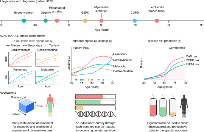
Model

We recapitulated the formulation of the model and provide a full account of model assumptions and implementation details.

Mathematical formulation

The ALADYNOULLI model represents the probability of disease occurrence for patient i, disease d, at time t via a mixture of probabilities as follows:

where κ is a global calibration parameter, θ_ikt represents patient i’s time-varying association with signature k, and ϕ_kdt captures the relationship between signature k and disease d over time.

The patient–signature associations θ_ikt are parameterized as a softmax function of latent variables λ_ikt as:

The ALADYNOULLI model is specified hierarchically, via distributional assumptions on many of these components, which we refer to as priors.

Indicating by λ^ik the function of time describing the evolution of the latent variable over time for patient i and signature k, we specify this as a Gaussian process:

where r^k is a signature-specific baseline, Γ^k captures how genetic and demographic factors g_i influence patient–signature associations, and Ω_λ is a kernel function controlling temporal smoothness. The covariate matrix G contains 36 PRSs plus sex and 10 genetic principal components (47 features total), providing genetic and demographic information for each individual. The kernel function Ω_λ is defined as:

In our implementation, the amplitude parameter α_λ is set to 100 and the length-scale parameter l_λ is set to T/4. Similarly, the disease–signature association temporal functions follow a Gaussian process:

where μ^d is a disease-specific baseline derived from the logit of the population prevalence, ψ_kd represents the the time invariant component of the association between signature k and disease d, and Ω_ϕ is a kernel function defined as:

where the amplitude is fixed to α_ϕ = 100 and the length scale is set to l_ϕ = T/3 in our implementation.

The genetic effect parameters Γ^k form a vector of length P representing the effects of P genetic, sex and ancestral covariates on signature k, and are assigned independent zero-mean Gaussian priors:

where \(\sigma _\gamma ^2\) is the prior variance.

Censored data and detailed E matrix formation methodology

A critical aspect of ALADYNOULLI is its careful handling of censored observations, which is part of what allows it to function as a generative model of disease progression rather than a retrospective analysis tool. The likelihood function, defined below, incorporates time-to-event information through a standard survival analysis encoding of binary disease-specific event indicators in Y and censoring times in E. Element E_id in E represents, in summary, the minimum of the disease-specific event time and the maximum follow-up time for the patient, ensuring that the likelihood only includes timepoints at which the patient was actually observed. This formulation properly accounts for competing risks by using censoring times derived from actual data.

More specifically, the matrix E is defined through the following steps:

Step 1: identify maximum follow-up time for each patient. For each patient i, we determined their maximum follow-up age from ICD-10 data: max censor_i = max(last diagnosis date_i, administrative censor date_i). This represents the last timepoint at which patient i could have been observed, accounting for death, loss to follow-up, emigration or end of study period.

Step 2: convert to timepoint scale. We converted the maximum censoring age to the timepoint scale of the model: max timepoint_i = max censor_i − 30, where timepoint 0 corresponds to 30 years of age.

Step 3: cap event or censor times in E matrix. For each patient i and disease d, the E matrix entry is as follows:

• If disease d is not observed in patient i, then E_id = max timepoint_i.

• If disease d is observed in patient i, then E_id is the age of the diagnosis of disease d for patient i in years, minus 30.

Step 4: apply to prevalence calculation. When computing prevalence at each age t, we only included patients who are still at risk:

where the denominator includes only patients who have not yet been censored at timepoint t. This ensures that prevalence estimates reflect realistic at-risk periods.

Likelihood function

The likelihood is constructed to respect this censoring structure^22,46. Consider first \(\mathcalL_NLL\), the negative log of the likelihood, that is, the negative log of the probability of observed disease histories conditional on the disease probabilities (π):

The contribution of individual i to this expression has three components:

1. (1)

   Pre-event survival (t < E_id): for all timepoints before the event or censoring time, we know that the individual did not have disease d, contributing log(1 − π_idt) to the likelihood at each time.

2. (2)

   Event occurrence (t = E_id, \(Y_idE_id=1\)): if disease d occurred at time E_id, we observed the event. The corresponding contribution is \(\log (\pi _idE_id)\).

3. (3)

   Censored observation (t = E_id, \(Y_idE_id=0\)): if the individual was censored without disease at time E_id, we only know they were disease free at that time, contributing \(\log (1-\pi _idE_id)\).

Objective function for maximum a posteriori computation

The computational derivation of the maximum a posteriori (MAP) estimate of the unknown parameters in the model proceeds by optimizing the function \(\mathcalL_total\), which includes the negative log-likelihood \(\mathcalL_NLL\) as well as terms arising from the Gaussian process prior.

The negative logs of the Gaussian process terms, as previously specified, are:

where μ^ik = r^k + Γ^k Gi. Combining these terms, and assuming diffuse near-uniform priors on κ and Γ, the negative log posterior (the ‘loss’ for short) is:

Training, validation and testing architecture

The genetic and performance results in this paper are based on training in the UKB dataset; we also trained the model in the MGB and AoU datasets to establish consistency as in Fig. 2. Model fit for all three datasets, including ϕ parameters, disease prevalence μ and primary time-fixed signature–disease associations ψ_k, is available in the exported parameters at the Zenodo deposit. Our analytical approach includes two complementary goals: (1) retrospective analysis for model training and cross-cohort validation; and (2) prospective analysis for prediction evaluation, as summarized in Extended Data Fig. 1.

Retrospective analysis

For computational efficiency and uncertainty quantification, we divided each cohort into non-overlapping subsets: the UKB into B = 40 subsets of approximately 10,000 individuals each (reserving each subset of 10,000 individuals in turn as a held-out test set), AoU into 30 subsets and the MGB into 4 subsets (reflecting the smaller dataset sizes). For each subset b within each cohort, we jointly estimated the disease–signature associations (\(\widehat\phi ^(b)\)) and individual loadings (\(\widehat\lambda ^(b)\)) using all available observed data up to 81 years of age or censoring time, whichever came first. This retrospective approach utilized the complete disease trajectory for each individual, enabling us to characterize the full spectrum of disease signatures and their temporal dynamics. For initialization, each subset uses the same pre-computed initial clusters and ψ parameters, facilitating consistent signature interpretations across all subsets within each cohort.

For the UKB, the final disease–signature parameters used for explanatory analyses were computed as the average across the 40 training subsets (excluding the held-out test set):

This subset-averaging approach provides robust parameter estimates while maintaining computational tractability. In addition, it facilitates assessment of estimation robustness. The AoU and MGB cohorts serve as external validation datasets, demonstrating the replicability of disease signatures across different populations and healthcare systems. No prediction tasks were performed on these two cohorts.

This subset-averaged ϕ was used to generate the disease signature visualizations in Fig. 2, including the temporal patterns and cross-cohort consistency analyses. Individual trajectory analyses (Fig. 3) utilized the subset-specific λ^(b) estimates, and subsequent clustering of patients by their time-averaged signature loadings was performed within each disease category. The genetic analyses (Fig. 4) were performed exclusively in the UKB, using the AUC of individual signature trajectories as quantitative phenotypes for GWAS.

Prospective analysis

For prediction evaluation (Fig. 5), we implemented a strictly prospective framework using only UKB data with leave-one-out cross-validation to ensure robust, generalizable performance estimates. We used a subset of 400,000 individuals (the first 400,000 participant IDs, which are random, in 40 batches of 10,000 each) from the full UKB cohort of 427,239 individuals for computational efficiency in the cross-validation framework. For each of the 40 batches, we trained models on the remaining 39 batches to learn population-level parameters: disease–signature associations (ϕ), signature offsets (ψ), genetic effects (γ) and the global calibration parameter (κ). These parameters were then fixed, and predictions for the held-out batch of 10,000 individuals were generated by learning only individual-specific trajectories (\(\widehat\lambda \)) using only data available up to specific prediction timepoints.

This approach ensures no information leakage from the held-out batch. It also reflects the intended real-world clinical scenarios where population-level disease patterns are known from previous research, but individual risk trajectories must be estimated from available clinical history up to the prediction time. All prediction performance metrics reported in this paper are based on this leave-one-out cross-validation approach.

Model initialization

To ensure computational feasibility and parameter stability, we initialized training as follows. We performed the spectral clustering of diagnoses described below and used it to derive starting values for ψ. We did this once on the entire dataset to establish stable disease clusters and signature–disease associations. These initial ψ values were then reused in all subsequent subset analyses for b = 1,…, 40.

Spectral clustering was performed using Scikit on disease co-occurrence patterns. We computed a disease co-occurrence matrix C where C_dd′ represents the frequency with which diseases d and d′ co-occur in the same patient. We applied spectral clustering to this matrix to identify K disease clusters.

We then initialized the ψ_kd parameters based on cluster membership: for diseases in cluster k, we set ψ_kd = 1.0 + ϵ where ϵ is a small random noise. For diseases not in cluster k, we set ψ_kd = −2.0 + ϵ. The choice of initial ψ was initialized at values of 1 and −2, which on the log scale correspond to a 20-fold difference in odds (that is, 10⁻⁹ versus 10⁻¹¹), thereby spanning a broad range of plausible values for disease risk. For the time-varying parameters λ_ikt and ϕ_kdt, we initialized by drawing a single sample from the corresponding Gaussian process prior with reduced variance to preserve the structured mean initialization. Specifically, we initialized λ_ikt via a random draw from the Gaussian process prior with mean \(\bfr_k+\boldsymbol\Gamma _k^\rm\top \bfg_i\) and covariance kernel scaled by amplitude α = 0.1, where Γ^k was initialized using regression on disease occurrences. We initialized ϕ_kdt via a random draw from the Gaussian process prior with mean μ^d + ψ_kd and the same reduced amplitude, where μ^d is derived from the logit of disease prevalence. The reduced amplitude ensures that random deviations do not bias the parameters arbitrarily away from the informative mean structure while maintaining temporal smoothness. We generated the Gaussian process samples via Cholesky decomposition of the scaled kernel matrices. This approach provides a structured and plausible initialization that reflects our prior smoothness assumptions. The number of latent signatures K was chosen to provide a parsimonious balance between model complexity and interpretability, based on previous experience and exploratory analysis.

Optimization details

We trained the model using gradient descent to minimize the loss (equation (6)). The solution can be interpreted as approximating a MAP estimate of the parameters, assuming dispersed priors on λ, Γ, μ, ψ and ϕ. We minimized the loss (equation (6)) over a fixed maximum number of epochs (that is, complete passes through the entire training dataset). At each epoch, we computed gradients via backpropagation and updated parameters using the Adam optimizer in PyTorch, a deep learning framework that allows efficient computation of gradients through automatic differentiation. The model was trained using a learning rate of 0.01. The model was optimized at a timescale of 1 year and thus trained to provide the most accurate 1-year risk predictions. Longer-term risk (for example, 10 years) can also be derived by simple manipulations of the estimated π.

For computational efficiency, we used the Cholesky decomposition to compute the Gaussian process contributions and to sample from the Gaussian process prior during initialization. We also used a jitter term of 1⁻⁶ to ensure numerical stability when computing the inverse of the kernel matrices. In practice, for our subsets of 10,000 individuals, the model converged after 200 epochs. For inference on new patients, the vectorized implementation enabled rapid risk prediction: generating predictions for a single individual requires approximately 0.05 s (or 8 min for 10,000 individuals), making the model suitable for real-time clinical decision support.

Computation of probabilities of future events

To ensure that our model provides prospective predictions without data leakage, we implemented a strict censoring strategy that distinguishes between cohort recruitment and prediction time. This approach allowed us to simulate real-world clinical scenarios where predictions are made based only on information available at a specific point in time (see Supplementary Fig. 1).

Cohort enrolment time refers to the timepoint when an individual enters ALADYNOULLI, which for our purposes is 30 years of age. For example, in our UKB analysis, all individuals were followed in the EHR from 1980 forwards^15,47 and thus assigned an enrolment time in our study at young adulthood, 30 years of age, or whichever comes later.

Cohort recruitment time refers to the time when individuals joined the biobank. The UKB recruited individuals between 40 and 69 years of age in the time frame from 2006 to 2010 (ref. ³).

Prediction time refers to the time when we imagine making a clinical prediction, with knowledge of the health history up until that time.

For prediction time for benchmarking with existing clinical risk scores, in practice, when comparing to existing clinical scores, this coincides with recruitment time as above.

In the UKB, an individual was observed in the EHR from adulthood and contributed data to our analysis from 30 years of age until the end of follow-up. However, for prediction analyses, we only made predictions at timepoints after the cohort recruitment time.

Simulation study

To validate the ability of the ALADYNOULLI model to recover latent disease clusters and temporal dynamics, we conducted a simulation study using ALADYNOULLI itself as the generative model. This approach allowed us to test whether the model can accurately recover known ground-truth parameters from synthetic data that follow the exact same probabilistic structure as our proposed model (Supplementary Fig. 23).

We generated synthetic data with N = 10,000 individuals, D = 20 diseases, T = 50 timepoints (30–79 years of age), K = 5 latent disease signatures and P = 5 genetic covariates. The data generation process followed the exact mathematical formulation of ALADYNOULLI. We first created K = 5 distinct disease clusters with 4 diseases per cluster, assigning strong positive associations within clusters (ψ_kd = 1.0) and strong negative associations outside clusters (ψ_kd = −2.0). Disease baseline trajectories (μ_d) were generated on the logit scale with diverse prevalence patterns ranging from rare (logit prevalence ≈ −14) to common (logit prevalence ≈ −8), incorporating realistic age-dependent onset patterns with varying peak ages and slopes.

For individual trajectories, we generated genetic covariates \(\bfG\in \mathbbR^N\times P\) and genetic effect matrices \(\Gamma \in \mathbbR^P\times K\), then sampled individual signature loadings λ_ikt from Gaussian processes with means \(\bfg_i^\rm\top \boldsymbol\Gamma _k\) and temporal covariance with length scale T/4 = 12.5 years. Disease–signature associations ϕ_kdt were sampled from Gaussian processes with means μ_d + ψ_kd and temporal covariance with length scale T/3 ≈ 16.7 years. Event probabilities were computed using the exact ALADYNOULLI formula: \(\pi _idt=\sum _k=1^K\rmsoftmax(\lambda _ikt)\cdot \rmsigmoid(\phi _kdt)\), and disease events were sampled from these time-varying probabilities.

When we applied ALADYNOULLI to these synthetic data, the model successfully recovered the composition of the signatures (adjusted Rand index = 0.843, normalized mutual information = 0.943), and accurately reconstructed the temporal trajectories and genetic effects.

Ethics statement

This study analysed coded or de-identified human research data from three biobanks under institutional review board (IRB) approvals at MGB. All research was performed in accordance with the relevant guidelines and regulations of each contributing biobank and the MGB Human Research Committee.

Analyses of MGB data were performed under MGB IRB protocol 2018P001236 (‘Cardiometabolic disease risk prediction and healthcare utilization using electronic health record-derived data and genomics’), which is active and approved for data analysis. All MGB participants provided written or electronic informed consent for research use of their biospecimens and EHR data before enrolment.

Analyses of UKB data were performed under MGB IRB protocol 2021P002228 (‘Analyses of cardiovascular diseases and related disorders using data from UK Biobank participants’), determined exempt by the MGB IRB. The UKB received ethical approval from the North West Multi-Centre Research Ethics Committee (REC reference 11/NW/0382), and all UKB participants provided informed consent at recruitment. This work was conducted under UKB application number 7089.

Analyses of AoU data were performed under MGB IRB protocol 2020P001737 (‘Data Analysis for All of Us Research Program’), determined by the MGB IRB to constitute analysis of de-identified data not meeting the definition of human participant research. The AoU obtained ethical oversight via its central IRB at the Vanderbilt University Medical Center Data and Research Center, and all AoU participants provided informed consent at enrolment.

No identifiable patient images, individually identifying records or new prospective biospecimen collections were generated by this study; all analyses were performed on coded or de-identified longitudinal data already collected by the three contributing biobanks under the consent procedures described above.

Cohorts

Data are drawn from three distinct biobanks: MGB, UKB and AoU. Each cohort is described in Supplementary Table 2 and below (Supplementary Fig. 2).

MGB

MGB is an integrated research initiative based in Boston, Massachusetts⁴. It collects biological samples and health data from consenting individuals at Massachusetts General Hospital, Brigham and Women’s Hospital and local healthcare sites within the MGB network. Since 1 July 2010, the MGB has enrolled more than 140,000 participants and extracted DNA from approximately 90,000 participants’ samples and 53,306 participants were genotyped by Illumina Global Screening Array (Illumina). All participants provided their informed written or electronic consent. EHR data are available on all participants from approximately 1990 (see Supplementary Fig. 2). We used a subset of 48,069 for whom EHR and genetic data were available. The cohort inclusion criteria: all individuals with available EHR and genetic data were included; no restrictions were placed on the number of visits or age at enrolment, as the model accommodates variable follow-up times through its censoring framework.

UKB

The UKB is a large-scale, population-based cohort that recruited over 500,000 participants 40–69 years of age between 2006 and 2010 from across the UK^3,48. The cohort includes extensive phenotypic data, biological samples and longitudinal follow-up of health outcomes. Genotyping was performed using the UK BiLEVE array or the UKB Axiom array, with subsequent imputation to the Haplotype Reference Consortium and UK10K reference panels. Participants were genotyped to investigate genetic contributions to various health and disease traits, with particular attention to the relationship between genetic variants and cardiometabolic diseases. Electronic health records are available, with the earliest diagnostic records extending back to 1980 (ref. ⁴⁹), providing diagnostic history well before the 2006–2010 recruitment window. We used the subset of 427,239 for whom genomic and EHR data were available. PRSs were obtained from an external set of controls²⁸.

AoU

The AoU research programme⁵⁰ is a large-scale cohort study designed to increase the representation of historically understudied populations in biomedical research. Since 2018, AoU enrolled adults (18 years of age or older) at more than 730 US sites. Of the more than 800,000 consented participants, more than 560,000 have completed core enrolment requirements, including health questionnaires and biospecimen collection. Data from these participants are continuously linked to EHRs, which capture ICD-9 or ICD-10, SNOMED (Systematized Nomenclature of Medicine and Clinical Terms) and CPT (Current Procedural Terminology) codes. Genetic data include array-based genotyping from 315,000 participants and whole-genome sequencing from 245,394 participants who were then available to contribute PRSs for downstream analyses.

Preprocessing and disease encoding

Following the approach of Jiang et al.¹⁶, we initially analysed 348 PheCode diseases from the UKB that were selected based on prevalence thresholds (1,000 or more occurrences) to ensure sufficient statistical power for comorbidity analysis. This threshold was chosen to balance disease coverage with statistical power: diseases with fewer than 1,000 occurrences would have insufficient power for reliable signature assignment. We focused on ICD-10 chapters A–N (disease chapters), excluding injury (S and T), poisoning, external causes of morbidity and mortality (V–Y), factors influencing health status (Z) and codes for special purposes (U). Disease records were mapped from ICD-10 or ICD-10CM codes to PheCodes using a standardized three-step procedure: (1) direct ICD-10-to-PheCode mapping using established PheCode definitions²⁴, (2) aggregation of related ICD codes to single PheCode categories, and (3) validation of mapping consistency across cohorts. To validate our findings across independent populations, we then applied the same disease selection strategy to AoU and MGB cohorts using their respective ICD coding systems. In AoU, we extracted ICD-9 and ICD-10 codes directly from the OMOP Common Data Model condition occurrence tables⁵⁰, successfully reproducing all 348 diseases from the UKB selection. In the MGB, we similarly used ICD-9 and ICD-10 codes, reproducing 346 of the 348 diseases for validation analyses. This multi-cohort approach enabled us to assess the generalizability of disease signatures across different healthcare systems and populations while maintaining consistency in the underlying disease definitions used for ALADYNOULLI model development and validation.

Analysis

Stability across subsets and cohorts

We empirically verified that ϕ estimates were highly stable across subsets. To assess robustness to natural variation in sample composition, we computed standard errors of ϕ parameters across all 40 training batches. Each batch represents 10,000 individuals with slight variation in composition across batches. For each ϕ parameter (signature–disease–time combination), we calculated the standard error of the mean as the standard deviation across batches divided by \(\sqrt40\). We observed small standard errors (mean s.e. = 0.0010, median s.e. = 0.0002, 95% of s.e. values ≤ 0.004), demonstrating the robustness of our disease–signature associations to batch-to-batch variation in sample composition (Supplementary Fig. 6).

To further assess the replicability of our disease signatures across different populations (shown in Fig. 2c), we performed cluster correspondence as follows (Fig 2d). We examined the correspondence between disease clusters identified in each biobank by creating normalized confusion matrices. For each pair of biobanks (UKB versus MGB and UKB versus AoU), we identified the set of diseases common to both biobanks, mapped each disease to its assigned cluster in each biobank based on posterior fitting (disease-to-signature assignments determined by the signature with maximum posterior association strength, argmax_k(ψ_kd)), created a cross-tabulation matrix showing the proportion of diseases in each UKB cluster that was assigned to each MGB or AoU cluster, and normalized the counts by row to show the distribution of cluster assignments.

We computed a composition preservation probability index to quantify cross-cohort correspondence. For each UKB cluster k, we identified its best-matching cluster in the comparison cohort (the cluster receiving the highest proportion of diseases from that UKB cluster). The composition preservation probability for cluster k is defined as:

where D_k,UKB is the set of diseases in UKB cluster k (determined by posterior ψ values, argmax_k(ψ_kd)), \(D_k^* ,\rmother\) is the set of diseases in the best-matching cluster k^* in the comparison cohort (also determined by posterior ψ values) and ∣⋅∣ denotes set cardinality. This metric represents the proportion of diseases in a UKB signature that also belong to its best-matching signature in the comparison cohort (that is, the intersection size divided by the UKB signature size, rather than the traditional Jaccard intersection over union). The overall cross-cohort similarity is the median of these cluster-specific similarities: J = median(J₁, J₂,…, J_K) across all UKB clusters. This metric ranges from 0 (no correspondence) to 1 (perfect correspondence), where higher values indicate stronger replicability of disease clustering patterns across populations.

This analysis revealed strong correspondence between clusters across biobanks (median composition preservation probability = 0.80), particularly for cardiovascular and malignancy signatures, suggesting robust biological patterns that transcend population differences.

For temporal pattern analysis, we performed a detailed comparison of the temporal patterns (ϕ trajectories) for diseases shared across all three biobanks, focusing on two key signatures: the cardiovascular signature (signature 5 in the MGB, signature 16 in AoU and signature 5 in the UKB) and the malignancy signature (signature 11 in the MGB, signature 11 in the AoU and signature 6 in the UKB). For each signature, we identified diseases assigned to that signature in all three biobanks, plotted the temporal patterns (ϕ values) for each shared disease, overlaid the average pattern across all three biobanks (grey dashed line in Fig. 2) and used consistent colours for each disease across biobanks to facilitate comparison. This analysis demonstrated consistency in the temporal patterns of disease risk across different populations, with shared diseases showing similar risk trajectories despite being modelled separately in each biobank.

Individual patient trajectory visualization

To illustrate the complex interplay between disease signatures in individual patients (shown in Fig. 2a), we analysed detailed trajectories for patients with multiple conditions.

For each selected patient, we created a three-panel visualization showing temporal signature loadings, a disease timeline with diagnosis timing and disease specific probabilities, and then contrasted with the time-averaged signature contributions.

Disease-specific trajectory and heterogeneity analysis

To systematically quantify differences in signature composition among patients with the same clinical diagnosis and understand disease progression heterogeneity and associated genetic architectures (Figs. 3f and 4b–d), we performed trajectory clustering analysis using the ALADYNOULLI model. For each disease of interest (for example, breast cancer, major depressive disorder and myocardial infarction), we implemented the following analysis pipeline.

Patient selection and temporal averaging

For each disease, we identified all patients who developed the condition and computed their time-averaged normalized signature loadings:

where θ_ikt is the signature loading for individual i, signature k and time t.

Patient clustering

We applied k-means clustering (k = 3) to the time-averaged signature loading matrix \(\bar\theta _ik\) to identify illustrative distinct patient subgroups within each disease category.

Trajectory visualization

We computed cluster-specific mean trajectories across individuals within the cluster \(\mu _ckt=\frac1\sum _i\in C_c\theta _ikt\) and visualized deviations from population reference as filled line plots for each timepoint: Δ_ckt = μ_ckt − ref_kt, where ref_kt represents the population-average signature loading.

Genetic architecture analysis

For each cluster, we computed mean PRSs across individuals in the cluster, and created heatmaps showing cluster-specific values of these scores. To quantify variability of PRSs among individuals with the same disease, we calculated Cohen’s d effect sizes for each PRS comparing in-cluster versus out-of-cluster distributions:

where \(\barX_\rmin\) and \(\barX_\rmout\) are the mean PRS values for patients within and outside each cluster, respectively, and s_pooled is the pooled standard deviation. Cohen’s d values of 0.2, 0.5 and 0.8 correspond to small, medium and large effect sizes, respectively, providing a standardized measure of genetic differentiation between patient subgroups.

For cluster c and signature k, \(C_ck^\rmSIG\) is the standardized difference in mean time-averaged signature loadings between individuals in cluster c and those in all other clusters. This measures how distinct each cluster is with regard to each disease signature. Similarly, for cluster c and PRS p, \(C_cp^\rmPRS\) is the standardized difference in mean PRS values between individuals in cluster c and those in all other clusters.

Statistical significance of cluster-level Cohen’s d was assessed by two-sided Welch’s t-tests comparing in-cluster versus out-of-cluster individuals on the corresponding time-averaged signature loadings (\(C_ck^\rmSIG\)) or PRS values (\(C_cp^\rmPRS\)). Equivalently, \(t=d\sqrtn_\rminn_\rmout/(n_\rmin+n_\rmout)\) with df = n_in + n_out − 2. Reported P values use Bonferroni correction across the 21 signatures × 3 clusters tested per disease (\(C_ck^\rmSIG\)) and across the PRS panel × 3 clusters tested per disease (\(C_cp^\rmPRS\)).

Deviation pathway heterogeneity analysis for myocardial infarction

As a supplementary analysis, to identify illustrative biological pathways to myocardial infarction using deviation-from-reference clustering, we performed the following supplementary analysis. For each individual with a myocardial infarction diagnosis, we extracted signature loadings (θ_ik(t)) over the 10-year window preceding the myocardial infarction event. We computed signature deviations by subtracting the population reference trajectory for each signature: \(\delta _ikt=\theta _ikt-\bar\theta _kt\), where \(\bar\theta _kt\) is the population mean signature loading at age t. This deviation-based approach removes age-related confounding and focuses on disease-specific patterns relative to expected population trajectories. For each patient, we computed a 105-dimensional feature vector (21 signatures × 5 timepoints) representing mean signature deviations across the 10-year pre-myocardial infarction window. Patients were clustered into pathways using k-means clustering (k = 4) on these deviation vectors. Pathway assignment was validated through: (1) cross-cohort replication in the MGB using identical clustering procedures, (2) comparison of precursor disease prevalence patterns across pathways, and (3) signature trajectory visualization to confirm coherence with established clinical patterns. Cross-cohort validation was performed by applying the UKB cluster centroids to the MGB cohort and comparing pathway sizes and disease enrichment patterns.

Genetic analysis of signature trajectories

For each individual i, we computed the temporal signature loadings θ_ik(t) for each signature k and timepoint t using the softmax transformation:

where λ_ik(t) is the latent score for individual i, signature k and time t. The softmax was computed across the signature dimension for each individual and timepoint. To summarize the overall exposure each individual to a given signature, we integrated the signature trajectory over time:

where T is the total number of timepoints. The resulting average signature exposure over time (AEX) for each signature was used as a quantitative phenotype for downstream genetic association analysis (Extended Data Fig. 6).

We performed GWAS using the AEX values as quantitative phenotypes. For each signature k, we tested for association between the AEX phenotype and genome-wide SNP genotypes. Association testing was performed using the REGENIE⁵¹ software (described below), which implements a two-step ridge regression approach for computational efficiency and control of population structure.

Genetic ancestry handling

All GWAS analyses included individuals of all genetic ancestries (not restricted to European ancestry), with population structure controlled through inclusion of the first 20 principal components of genetic ancestry as covariates. This approach allowed us to leverage the full diversity of the UKB while properly accounting for population stratification. The following covariates were included in all association models: sex, age at recruitment and the first 20 principal components of genetic ancestry³.

GWAS details

We performed GWAS using REGENIE⁵¹, a two-step ridge regression approach designed for computational efficiency and robust control of population structure in large biobank-scale datasets.

Step 1: whole-genome ridge regression. We fit a whole-genome ridge regression model using all genetic variants to account for polygenic effects, relatedness and population structure. The model was fit using leave-one-chromosome-out cross-validation, where predictions for each chromosome exclude variants from that chromosome to prevent overfitting. This step produces polygenic predictions that capture the aggregate genetic background.

Step 2: single-variant association testing. We performed single-variant association tests on the residuals from step 1, testing each of 6,418,439 imputed variants (MAF ≥ 0.01, INFO ≥ 0.7) individually. By testing variants on pre-adjusted residuals rather than on raw phenotypes, this approach provides well-calibrated association statistics that are robust to case–control imbalance, relatedness and population stratification. All models included covariates for sex, age at recruitment and the first 20 principal components of genetic ancestry. Genome-wide significance was set at P < 5 × 10⁻⁸. We identified nearby genes using both nearest gene and gene body analyses (Ensembl and GnomaAD).

In addition to our main analysis featured in Fig. 4, for each signature, we identified genome-wide significant SNPs (for example, P < 5 × 10⁻⁸) and further analyse their relationships with individual disease phenotypes and nearby genes. The analysis proceeds as follows. First, we extracted the lead SNPs from the GWAS summary statistics for each signature. For our supplementary analyses (Supplementary Fig. 13), for each top SNP, we tested its association with a panel of binary constituent disease phenotypes, which comprise our signature inputs using logistic regression, controlling for sex and the first 20 principal components. Third, we visualized the matrix of SNP–phenotype association strength (−log₁₀(P)) using heatmaps, marking associations significant at P < 5 × 10⁻⁸. This enabled identification of signature-specific loci: SNPs associated with the signature but not with any individual constituent disease. Fourth, we used UpSet plots to visualize the overlap of significant variants across signatures and individual diseases.

LDSC heritability analysis

Heritability estimates (h²) represent the proportion of phenotypic variance in signature trajectories that can be attributed to additive genetic variation. Because our signature phenotypes are continuous (integrated area under the signature loading curve), all heritability estimates are on the observed scale, that is, there is no liability-scale transformation for continuous traits.

Heritability estimates for signature trajectories were calculated using linkage disequilibrium score regression (LDSC)³⁰ on the GWAS summary statistics generated from REGENIE. For each signature, we applied LDSC with standard parameters using the European ancestry linkage disequilibrium reference panel (baseline LD v2.2), following standard practice for heritability estimation from GWAS summary statistics. The LDSC intercept was used to assess potential residual confounding and genomic inflation. For comparison with component diseases, we also performed GWAS for individual cardiovascular traits (myocardial infarction, coronary artery disease, angina pectoris, hypercholesterolaemia, coronary atherosclerosis, acute ischaemic heart disease, chronic ischaemic heart disease and unstable angina) using the same REGENIE workflow and covariates (sex, age at recruitment and first 20 genetic principal components), then computed LDSC heritability estimates for each trait. For valid comparison, we have reported observed-scale heritability for binary traits; liability-scale estimates are provided separately for reference against literature values that typically report on that scale (Supplementary Table 5).

RVAS

Gene-based RVAS were performed using REGENIE⁵¹ gene-based association tests. For each signature, we tested associations between signature AEX values and aggregated rare variant burden within genes across six variant filtering masks (Mask1–Mask6), representing progressively inclusive functional impact categories (Mask1: most restrictive, Mask6: most inclusive). Each mask was further stratified by MAF thresholds (singleton, 1 × 10⁻⁵, 0.0001, 0.001, 0.01 and 0.1). Variants were annotated using Ensembl Variant Effect Predictor and aggregated at the gene level as well as Encode using nearest gene. The gene-based test statistic aggregates variant-level association signals within each gene, accounting for linkage disequilibrium and variant effect sizes. Genome-wide significance was set at P < 2.5 × 10⁻⁶ after Bonferroni correction for the number of genes tested per signature (18,464 genes); all reported significant gene–signature pairs additionally satisfy the joint Bonferroni threshold P < 0.05/(18,464 × 21) ≈ 1.3 × 10⁻⁷ controlling for the 21 signatures considered. Significant genes were identified across all masks to ensure robustness to variant filtering criteria, with genes discovered in multiple masks considered high-confidence associations.

Three-way validation of rare variant associations

To validate rare variant associations through an independent pathway, we examined the three-way consistency between (1) signature–gene associations from RVAS, (2) gene–disease correlations from rare variant burden analysis, and (3) disease–signature loadings from the ϕ parameters. For each signature–gene pair identified through RVAS, we computed rare variant burden scores for each individual by summing variant counts (burden = ∑(2 − X), where X is the genotype matrix with PLINK encoding. We then calculated Pearson correlations between rare variant burden and binary disease outcomes across all diseases. Finally, we tested whether diseases with high rare variant burden correlations also showed high signature–disease loadings (ϕ values) by computing the correlation between the vector of gene–disease correlations and the vector of disease–signature loadings. This three-way validation provides biological plausibility by demonstrating that: (1) rare variant carriers show disease enrichment consistent with signature associations, and (2) signature–disease loadings reflect the same underlying biology captured by rare variant–disease associations.

Clinical validation: familial hypercholesterolaemia and clonal haematopoiesis

To validate signature concordance with established disease biology, we performed targeted analyses of two well-characterized genetic conditions with known disease associations. For familial hypercholesterolaemia, we identified carriers of familial hypercholesterolaemia using genetic variants in LDLR, APOB and PCSK9 following an established criteria^52,53,54. For carriers of familial hypercholesterolaemia and matched controls, we computed signature loadings and tested for enrichment of signature 5 (cardiovascular signature) in the 5-year window preceding the first ASCVD event (myocardial infarction, coronary artery disease or stroke). For each patient with an ASCVD event, we computed the pre-event change in signature 5 loading (ΔSig5) over the 5-year window preceding the event, defined as the difference between signature loading at 1 year before the event and at 5 years before the event. We then classified patients as showing a ‘pre-event rise’ if ΔSig5 ≥ 0. Enrichment was quantified by comparing the proportion of carriers of familial hypercholesterolaemia versus non-carriers who showed a pre-event rise using Fisher’s exact test on a 2 × 2 contingency table (rise/no-rise × carrier/non-carrier), two-sided alternative. Results were reported as odds ratios with P values from Fisher’s exact test.

Model evaluation and comparison

Figure 5 presents a comprehensive evaluation of our multi-disease risk prediction model in the UKB, and comparisons with important single-disease models. Each was evaluated in a strictly prospective framework that minimizes known sources of information leakage. In the testing data, all individual-level parameters were estimated using only information available up to the time of prediction. Individuals with prevalent disease at prediction were excluded from the risk set for that disease. In the UKB, all individuals were followed for at least 10 years from recruitment. We considered the following prediction tasks and metrics.

Median AUC ALADYNOULLI dynamic

This metric evaluates the ability of the model to make dynamic predictions at multiple timepoints during follow-up: it is derived by refitting the ALADYNOULLI model using fixed \(\widehat\phi \), \(\widehat\gamma \) and κ parameters, previously estimated from the full history training data, and now applied to a series of 1-year prediction tasks. Critically, although the fixed parameters above were estimated from the full training data, the \(\widehat\lambda \) for each prediction task were estimated using data only up to the point of prediction. For each of the first 10 years after recruitment, the model was retrained using only data available up to that point for the held-out test set (in orange in Extended Data Fig. 1). The median AUC across these ten dynamic 1-year fits is reported. This captures how predictive accuracy evolves as patients accumulate new diagnoses and leverages the flexibility of our method to perform dynamic, prospective risk estimation at any timepoint. Individuals with prevalent disease at prediction time were excluded from the risk set.

ALADYNOULLI recruitment (1 year)

This metric uses the ALADYNOULLI model’s predicted 1-year risk at the time of recruitment, evaluated against observed 1-year outcomes. The risk estimate is \(\widetilde\pi _idt\), the predicted 1-year risk for individual i recruited at time t for disease d. In practice, any age of prediction could be chosen, but we used the age of recruitment to the UKB because it is the only time at which we have the availability of additional clinical variables required for comparability with existing clinical benchmarks.

ALADYNOULLI recruitment (10 years)

This metric uses the ALADYNOULLI model’s predicted 1-year risk at the time of recruitment, evaluated against observed 10-year outcomes. The risk estimate is \(\widetilde\pi _idt\), as in the 1-year predictions.

Cox

For benchmarking purposes, we used a baseline Cox model using only family history and sex as covariates, with age as the timescale delineating start and stop of the interval, representing a minimal clinical model that does not require any model curation or disease-specific features. This highlights the fact that our approach does not rely on disease-specific risk factors or manual feature engineering.

When benchmarking AUC performance, we compared the ALADYNOULLI model not only to the benchmarking Cox proportional hazards model above but also to established clinical risk scores: PREVENT⁵⁵, PCE⁵⁶ for ASCVD and Gail³⁹ for breast cancer, models for diseases for which these scores are available after specific and often expensive curation. Of note, these clinical risk scores require laboratory values and biomarkers that are either collected during targeted clinical visits (introducing selection bias) or, when extracted from routine EHR data, may be subject to measurement bias as patients who are sicker typically receive more frequent testing. By contrast, our approach leverages routinely collected diagnostic codes (ICD codes) that are systematically recorded for all patients regardless of disease severity, providing a more unbiased data source for risk prediction.

This approach ensured that all model comparisons were fair, prospective and reflective of the information available at the time of risk assessment.

Dynamic 10-year rolling

This approach demonstrates the interpolation capabilities of the model by evaluating how probability estimates evolve as new information becomes available. For each year of the 10-year horizon, we updated the predictions of the model using information available up to that timepoint, then aggregated the cumulative 10-year risk as \(1-\prod _t=1^10(1-\widehat\pi _idt)\), where \(\widehat\pi _idt\) is the predicted risk for individual i and disease d at year t after recruitment. Although this rolling evaluation does not use knowledge of the future outcome of interest, it cannot be considered fully prospective. This is because it incorporates concurrent information about events that are potentially correlated with, or even resulting from, the event of interest, as the probability estimates of the model at year t are influenced by information available up to year t. Thus, it is best understood as interpolation rather than extrapolation. Although this metric cannot be used for prospective evaluation, it demonstrates the technical capabilities of the model for dynamic risk assessment and shows how probability estimates evolve over time.

Additional methodological challenges

We conducted a series of analyses to assess the robustness of ALADYNOULLI to selection bias, population stratification, temporal leakage and reverse causation, complementing the primary analyses described in the main text. We provide technical details next.

Three key methodological features were included: (1) inverse probability weighting (IPW) to correct for UKB participation bias while preserving biological signal; (2) comprehensive washout analyses (1–6 months and 1–-2 years) to assess temporal leakage and reverse causation; and (3) patient-specific censoring using realistic follow-up times to properly handle competing risks. These strengthen the validity and generalizability of our findings.

Selection bias and IPW

To evaluate robustness to participation bias in the UKB, we implemented IPW following Schoeler et al.³⁸. We fit a lasso-regularized logistic regression model for biobank participation using demographic and socioeconomic variables (region, birth year, sex, household characteristics, employment status, housing tenure, ethnicity, self-reported health and education) and computed the predicted participation probability \(\widehatp_i\) for each individual.

IPWs were defined as

where 4.34% is the estimated participation rate in the source population, with \(w_i^* \) trimmed at the 1st and 99th percentiles to avoid undue influence of extreme weights. These raw weights were then normalized to sum to N:

ensuring that the weighted sample size equals the observed sample size for proper loss scaling.

The weighted loss function modifies the data likelihood component of equation (6) to incorporate individual weights. The weighted negative log-likelihood is:

where w_i is the normalized IPW weight for individual i. The Gaussian process prior terms (\(\mathcalL_\rmGP\lambda \) and \(\mathcalL_\rmGP\phi \)) remain unweighted, as they represent priors on model parameters rather than data contributions.

This formulation ensures that individuals with lower predicted participation probabilities (underrepresented groups) contribute proportionally more to parameter estimation, effectively rebalancing the training data towards the source population distribution.

Population stratification and genetic ancestry

To assess the effect of population structure on signatures, we performed both principal component-adjusted and ancestry-stratified analyses. First, we compared models fit with versus without genetic principal components in the Gaussian process mean for λ (equation (3)), holding all other settings fixed. Disease–signature associations (ϕ) were nearly identical between models (correlation = 1.000, mean absolute difference < 0.002), demonstrating that disease–signature relationships are robust to principal component adjustment. By contrast, individual signature loadings (θ) showed ancestry-specific shifts, with cardiovascular signature 5 exhibiting the largest deviation for South Asian (SAS) individuals, consistent with known elevated cardiovascular risk in this group. Second, we performed principal component analysis on time-averaged signature loadings and examined clustering by ancestry (European (EUR), African (AFR), East Asian (EAS) and SAS), finding substantial overlap between groups with modest deviations along principal components for AFR, EAS and SAS. Finally, we compared ALADYNOULLI predictions to Cox baseline models including age, sex and genetic principal components, confirming that ALADYNOULLI retains a performance advantage across ancestry groups, indicating that its gains are not explained by ancestry covariates alone.

Reverse causation assessment: short-term washout

To test whether predictions are driven by diagnostic cascades immediately preceding events, we excluded events occurring within 1, 3 and 6 months of enrolment. Performance remained robust with minimal AUC degradation (mean drop = 0.0112 for 1-year predictions and 0.0010 for 10-year predictions), indicating that ALADYNOULLI captures predictive signal rather than reverse causation effects.

Temporal leakage assessment: multi-year washout

To address temporal misalignment between ICD-10 dates and true disease onset, we conducted two complementary analyses. First, we compared 10-year predictions made at enrolment with versus without excluding the first year of outcomes following enrolment. This analysis (Supplementary Fig. 19b) demonstrates robustness to excluding the first year of outcomes, with minimal performance degradation (for example, ASCVD AUC = 0.723 with 1-year exclusion versus 0.733 baseline). Second, we evaluated 1-year predictions at fixed timepoints (enrolment + 1 to enrolment + 9 years) using models trained with different washout periods (0, 1 and or 2 years). For each prediction timepoint t_pred ∈ 1, 2,…, 9, we trained models using data up to t_pred − w years, where w ∈ 0, 1, 2 represents the washout period. This analysis (Supplementary Fig. 19c) tests for temporal information leakage by varying the amount of training data available, demonstrating substantial residual predictive power even with 1–2-year washout periods across key diseases.

All analyses were performed using Python, with survival models implemented in lifelines and scikit-survival, and validated in R (v4.0) using the Survival package, and calibration and discrimination metrics computed using standard epidemiological methods.

Reporting summary

Further information on research design is available in the Nature Portfolio Reporting Summary linked to this article.