


Study population
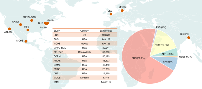
The genetic discovery analysis of TG:HDL ratio encompassed multiple cohorts with a cumulative sample size of 1,032,116 participants. Study participants were recruited from various population-based and hospital-based health systems across three continents (Fig. 1 and Supplementary Table 1). These cohorts included: the UK Biobank population-based study (UKB, n = 409,602)60; the Geisinger Health System MyCode cohort (GHS, n = 143,129)61; the Mexico City Prospective Study (MCPS, n = 136,725), a study of residents in two districts of Mexico City (Coyoacán and Iztapalapa)62 with a genetically admixed population with components of Indigenous American, European and African ancestry as described in detail previously63; the Mayo Clinic Project Generation health system-based cohort (MAYO-RGC, n = 80,941)64; the population-based BangladEsh Longitudinal Investigation of Emerging Vascular and nonvascular Events (BELIEVE, n = 69,663)65; the Colorado Center for Personalized Medicine biobank, a health system-based cohort (CCPM, n = 56,173)66; the UCLA ATLAS Precision Health Biobank, a health system-based cohort (ATLAS, n = 45,533)67; the Mount Sinai BioMe BioBank, a health system-based cohort (BioMe, n = 45,440)68; the University of Pennsylvania Penn Medicine BioBank, a health system-based cohort (PMBB, n = 25,785)69; the population-based Dallas Biobank Study at UT Southwestern Medical Center (DBS, n = 13,979)70; and the population-based Malmö Diet and Cancer Study (MDCS, n = 5,146)71. Analyses of other cardiometabolic phenotypes included participants from the aforementioned cohorts and also 4,755 participants from the Indiana University School of Medicine (Indiana-CLDB) study and 53,325 participants from the South Asia Biobank72. All studies received approval from the relevant ethics committees as listed below, and the participants gave their informed consent to take part in the research. UKB cohort: ethical approval for the UKB was obtained from the North West Centre for Research Ethics Committee (11/NW/0382). The work described here was approved by the UKB under application number 26041. GHS cohort: The MyCode Community Health Initiative was approved by the Geisinger institutional review board (IRB; study 2006-0258). MCPS cohort: the study was approved by scientific and ethics committees within the Mexican National Council of Science and Technology (0595 P-M), the Mexican Ministry of Health and the Central Oxford Research Ethics Committee (C99.260). MAYO-RGC cohort: the study was approved by the Mayo Clinic IRB under protocol number 09-007763. BELIEVE cohort: BELIEVE has received approvals from the relevant institutional review boards of the Bangladesh Medical Research Council, the National Heart Foundation Hospital and Research Institute, icddr,b and Bangabandhu Sheikh Mujib Medical University (BMRC/NREC/2013- 2016/390; BMRC/NREC/2016-2019/243; BSMMU/2019/1184; BSMMU/2019/1185; PR-18051; HBREC.2019.09). CCPM cohort: biospecimens and associated data used in this study were obtained from the biobank at the Colorado Center for Personalized Medicine (CCPM) at the University of Colorado Anschutz Medical Campus (CU AMC). All samples and data were collected under IRB approved protocol (15-0461). ATLAS cohort: ATLAS is an approved study by the University of California Los Angeles (UCLA) IRB (UCLA IRB 17-001013). BioMe/Mount Sinai Million Health Discoveries Program: The Icahn School of Medicine at Mount Sinai’s IRB, Program for the Protection of Human Subjects (PPHS), approved the BioMe Biobank and Mount Sinai Million Health Discoveries Program (PPHS IRB 11-01139 and 21-01743). PMBB cohort: the PMBB is approved by the University of Pennsylvania IRB under protocol number 813913. DBS cohort: The University of Texas Southwestern (UTSW) Biobank was reviewed and approved by the UTSW IRB under the study STU 022011-116: “Genetic Variation in a Multi-Ethnic Population”. MDCS cohort: IRB approval for MDCS was obtained from the Ethics committee of Lund University (LU 51-90) and the Regional Board of Ethics in Lund (Dnr 2016/479). Indiana-CLDB: the study has been reviewed by Indiana University IRB and approved under the protocol number 1105005445. South Asia Biobank: the study received ethical approval from the institutional Research Ethics Committee (18IC4698).
Clinical phenotypes
Clinical biomarkers
Measurements of blood lipids, glycaemic markers, transaminases, CRP and blood pressure were obtained either through direct clinical assessments or electronic health record (EHR) extraction, depending on the cohort type. For participants in population-based cohort studies, these measurements were conducted during standardized visits to designated assessment centres. By contrast, for participants from health-system-based cohorts, data were extracted retrospectively from EHR datasets and participant-specific median values were used. Blood lipid levels were primarily assessed using routine clinical chemistry methods across most cohorts. In the MCPS and BELIEVE studies, lipid measurements were derived from nuclear magnetic resonance metabolomics profiling, performed using the Nightingale Health platform73. Blood lipids were corrected for medication use by dividing by a class-specific correction factor obtained from previously reported clinical trials19,74,75,76,77,78. The TG:HDL ratio was calculated using triglyceride and HDL cholesterol values obtained from the same blood draw at baseline in epidemiological cohort studies (5 cohorts and 635,115 participants). In EHR-based studies (6 cohorts and 397,001 participants), where multiple measurements were available, median values across clinical encounters were calculated for TG and HDL separately and then the ratio of the median values was calculated. The use of median values across encounters is a standard approach in EHR-based genetic research to define a patient’s typical lipid profile79,80,81. Importantly, this avoids the exclusion of participants with valid but non-concurrent lipid measurements, thereby preserving sample size and discovery power. A sensitivity analysis was conducted restricting the TG:HDL ratio to values derived from TG and HDL measured concurrently from the same blood draw. A stratified analysis by fasting status was also conducted in the UKB, comparing TG:HDL ratios derived from fasting samples (defined as at least 6 h since the last meal) with those from non-fasting samples (defined as at most 2 h since the last meal). Blood pressure levels were corrected by adding 15 mmHg to systolic and 10 mmHg to diastolic blood pressure in those individuals receiving anti-hypertensive treatment as previously reported82.
Liver biopsy
The bariatric surgery cohort at Geisinger Health System (GHS) comprises 3,599 participants of European ancestry who underwent bariatric surgery procedures61. Intraoperative wedge liver biopsies were systematically obtained 10 cm left of the falciform ligament before any manipulation of the liver or stomach. Biopsies were sectioned, with the principal portion allocated for clinical histopathology—fixed in 10% neutral buffered formalin and stained with haematoxylin and eosin for general assessment and Masson’s trichrome for fibrosis evaluation. The remaining tissue was preserved in a research biobank, either stabilized in the RNAlater tissue collection system (Thermo Fisher Scientific) or snap-frozen in liquid nitrogen. Histopathological evaluation was conducted by an experienced pathologist and independently reviewed by a second pathologist. Scoring followed the Nonalcoholic Steatohepatitis Clinical Research Network (NASH CRN) system83, with steatosis graded as 0 (<5% parenchymal involvement), 1 (5 to <34%), 2 (34 to <67%) or 3 (>67%); lobular inflammation as 0 (none), 1 (mild, <2 foci per ×200 field), 2 (moderate, 2–4 foci per ×200 field) or 3 (severe, >4 foci per ×200 field); hepatocyte ballooning as 0 (none), 1 (few ballooned cells), or 2 (many/prominent ballooned cells); and fibrosis staged from 0 (none) to 4 (cirrhosis) according to established criteria. The MASLD activity score was generated by summing of the steatosis, lobular inflammation and ballooning scores.
Imaging phenotypes
MRI
MRI images were obtained from the UKB imaging cohort. For quantification of liver fat, we used data from a two-dimensional abdominal MRI scan that included the liver; a subset of individuals was scanned using a Dixon gradient echo protocol, while those imaged from 2016 onward were scanned using the IDEAL (iterative decomposition of water and fat with echo asymmetry and least-squares estimation) protocol. The resulting data have an in-plane pixel size of 2.5 × 2.5 mm and a slice thickness of 6 mm.
Whole-body MRI scans, spanning from the neck to the knees, were obtained through a two-point Dixon84 spoiled gradient-echo (FLASH) T1-weighted protocol with echo times of 2.39 ms (out of phase) and 4.77 ms (in phase), a repetition time of 6.69 ms and an excitation flip angle of 10 degrees85. Image acquisition was split across six distinct anatomical stages, each representing a separate 3D volume, with an in-plane spatial resolution of 2.23 mm × 2.23 mm and an out-of-plane resolution ranging from 3.00 mm to 4.50 mm according to the specific stage.
All images were captured using Siemens MAGNETOM clinical MRI scanners (Siemens Healthineers).
MRI-derived phenotypes
To assess total body adipose tissue volumes, we used an automatic segmentation model developed to delineate major adipose depots from Dixon MRI data into visceral and subcutaneous compartments86; visceral fat was further subdivided into mediastinal and abdominal components, and subcutaneous fat into the upper-body, abdominal and gluteofemoral components. The volume of fat within these regions was computed by summing the fat fractions for voxels within the segmented regions. The visceral-to-gluteofemoral fat ratio—a marker associated with poor metabolic outcomes9—was computed as the abdominal visceral fat volume divided by the subcutaneous gluteofemoral fat volume; the abdominal-to-gluteofemoral subcutaneous fat ratio was similarly computed using the respective total volumes. All data processing and phenotype extraction was conducted using the UKB Research Analysis Platform.
The liver fat percentage, measured as proton density liver fat fraction (PDFF), represents the proportion of fat content in the liver. A deterministic image processing algorithm was used to segment the liver on MRI images, using a multithresholding approach to exclude vessels. The methodology was validated using a publicly available phantom dataset containing vials with varying fat concentrations. PDFF within the segmented region was determined as the ratio of fat signal to the total fat and water signals16,87. To account for any systematic differences between PDFF estimates from gradient echo and IDEAL, the mean values were shifted to be equal for the two modalities, and an indicator variable encoding the imaging modality was included as an additional covariate for genetic analyses to account for any residual differences.
BIA
BIA for body composition was performed at the baseline using the Tanita BC 418ma Body Fat Analyzer. Fat and fat-free mass estimates derived from BIA were obtained from UKB fields 23100 and 23101, respectively; these are defined such that fat-free mass is equal to total body weight minus fat mass. The body fat percentage was calculated using the BIA-derived fat mass and baseline weight (UKB field 23098).
DEXA
DEXA measures were obtained using the GE-Lunar iDXA instrument. DEXA-derived measures of lean mass and android/gynoid fat mass were obtained from the UKB (UKB fields 23280, 23245 and 23262 respectively).
Disease definitions
Type 2 diabetes
Individuals diagnosed with type 2 diabetes were ascertained according to established methodologies9. Case identification was based on the presence of (1) at least one inpatient or two outpatient EHR entries with type 2 diabetes diagnosis codes (ICD-10: E11, O24.1; or ICD-9 equivalents), or documentation as a cause of death; (2) glycaemic biomarker measurements (HbA1c, random or fasting glucose) consistent with the diabetic range88 or algorithmically defined type 2 diabetes status derived from self-reported medical history and medication use89. Participants were excluded from cases if they met criteria for type 1 diabetes, indicated by ICD-10 codes E10, O24.0 or algorithmic classification based on self-reported and medication data89. Control participants were those not fulfilling type 2 diabetes criteria, with further exclusions applied for any EHR evidence of diabetes (any type), family history of diabetes or glycaemic biomarkers within the prediabetic range.
Liver disease
Cases of liver disease, encompassing MASLD and liver cirrhosis, were identified according to previously reported criteria16. Case inclusion required fulfilment of at least one of the following: (1) documentation of liver disease in EHRs from at least one inpatient encounter, two or more outpatient encounters or as a recorded cause of death; (2) self-reported diagnosis at the baseline; or (3) documented history of surgical or medical interventions related to liver disease. Individuals not meeting these criteria were classified as controls. Exclusion from the control group was applied if any of the following were present: (1) diagnosis of a liver disease not qualifying as a case; (2) outpatient encounter for the liver disease of interest; (3) elevated ALT levels (>25 IU l−1 in women, >33 IU l−1 in men); or (4) diagnosis of ascites attributed to liver pathology.
CAD
Cases of CAD were identified according to previously described criteria9. Inclusion as a case required fulfilment of at least one of the following: (1) documentation of CAD and/or myocardial infarction in EHRs from at least one inpatient encounter, two or more outpatient visits or as a recorded cause of death; (2) self-reported diagnosis of CAD or myocardial infarction at the baseline; or (3) documented history of surgical or medical interventions for CAD, including coronary artery bypass grafting or percutaneous coronary intervention. Individuals not meeting case criteria were classified as controls. Control samples were further excluded if a family history of CAD was identified, on the basis of EHR or self-reported information at the study baseline.
Epidemiological analysis methods
The associations between the TG:HDL ratio and various phenotypes—including body weight, fat distribution, glycaemic indices, hepatic steatosis, liver injury markers and histopathological features—were estimated using correlation or linear regression models. TG:HDL ratio levels were stratified in percentiles. Cox proportional hazards models were used to estimate the time-to-event relationship between the TG:HDL ratio and the incidence of type 2 diabetes, myocardial infarction, MASLD and liver cirrhosis in at-risk individuals, that is, without the outcome at or before baseline.
DNA preparation and exome sequencing
As previously outlined90, genomic DNA (gDNA) libraries were constructed by enzymatically fragmenting high-molecular-mass DNA to achieve an average fragment length of 200 bp. To facilitate multiplexed exome capture and sequencing, unique 10 bp asymmetric barcodes were incorporated into the DNA fragments of individual samples during library amplification. Equimolar quantities of these barcoded libraries were combined and subjected to exome capture using either a modified xGen Exome Research Panel probe library (Integrated DNA Technology) or a modified version of the human comprehensive exome panel (Twist Bioscience). After PCR amplification and quantification, the enriched libraries were multiplexed and sequenced on Illumina platforms, generating 75 bp paired-end reads. Sequencing was performed on the Illumina HiSeq 2500 and NovaSeq 6000 instruments, using S2 or S4 flow cells.
Read mapping and variant calling
Sequencing reads in FASTQ format were generated from Illumina image data using bcl2fastq (v.2.19.0) (Illumina). In accordance with the original quality functional equivalent (OQFE) protocol91, reads were aligned to the GRCh38 reference genome using BWA MEM (v.0.7.15)92 in an alt-aware configuration. Duplicate reads were identified and flagged, and additional per-read annotations were incorporated. Variant detection was performed using a Parabricks-accelerated implementation of DeepVariant (v.0.10), using a custom model to call single-nucleotide variants and short insertions and deletions, resulting in per-sample genome variant call format (VCF) files93. These individual VCF files were subsequently merged using GLnexus (v.1.4.3)94 to produce a joint-genotyped, multisample cohort-level VCF (pVCF). For downstream analyses, PLINK (v.1.9)95 was used to convert the pVCF file into PLINK-compatible files.
Exome sequencing quality control
For each cohort, we performed exome sequencing quality control with the following parameters: sample missingness <10%, variant missingness <10%, ±10 bp buffer window around target regions, a low heterozygosity HWE P > 1 × 10−100 and an excess heterozygosity HWE P > 1 × 10⁻³⁰.
Variant annotation
Variant annotation was performed using Variant Effect Predictor (VEP, v.100.4)96, using Ensembl release 100 human protein-coding transcript models97. For all analyses, a single functional consequence was assigned to each variant on the basis of its annotation on the canonical transcript. The canonical transcript for each gene was determined using a combination of MANE98, APPRIS99 and Ensembl canonical tags, following previously described procedures98.
Nonsense-mediated decay (NMD) predictions were performed using the NMD plugin in VEP96. A variant was predicted to escape NMD if it satisfies any of the four canonical rules: (1) the variant is located in the last exon of the transcript; (2) the variant is located within 50 bases upstream of the penultimate (second to last) exon; (3) the variant is located within the first 100 coding bases of the transcript; and (4) the transcript is intronless, containing only a single exon. A variant is predicted to escape NMD if it satisfies any of these four rules100,101.
Genetic association analyses
Genetic association analyses were conducted in each cohort using the linear whole-genome regression approach implemented in REGENIE (v.3.4 or older)102. Two primary analyses were performed across autosomes (chromosomes 1–22) and chromosome X in the discovery cohort: a genome-wide association study (GWAS) of common TOPMed- imputed variants103 (AAF ≥ 1%) and a gene-based association analysis of rare coding variants. In the first step of REGENIE (trait prediction based on genetic data), directly genotyped variants were included if they had an AAF ≥ 1%, missingness < 10%, Hardy–Weinberg equilibrium P > 10−15 and passed linkage disequilibrium (LD) pruning (window size, 1,000 variants; sliding window, 100 variants; r2 threshold, 0.1). The association model in the second step of REGENIE incorporated the following covariates: age, age2, sex, age × sex, age2 × sex, the first 10 principal components (PCs) based on common variants (derived from a set of LD-pruned array variants: 1,000-variant windows, 50-variant step size, r2 threshold 0.1), the first 20 PCs based on rare variants (the same pruning parameters) and cohort-specific sequencing batch covariates. The second step of REGENIE also included as a covariate a genome-wide leave-one-chromosome-out polygenic score generated in step 1, which adjusts for relatedness and residual population stratification102. For each variant or gene burden being tested in step 2, the polygenic score used leaves out the chromosome of the variant or the gene burden being tested (https://rgcgithub.github.io/regenie/)102. The main analysis was a pooled multiancestry analysis (that is, not stratified by ancestry). We also separately performed sensitivity analyses stratified by ancestry (that is, European, admixed American, South Asian, African and East Asian ancestries). For the non-pseudoautosomal regions of chromosome X, a dosage compensation model was used: homozygous reference males were coded as 0, hemizygous males as 2 and heterozygous males set as missing.
To ensure independence between rare and common variants signals in the same chromosome, exome-wide gene-burden analyses were additionally adjusted for common variant signals (minor allele frequency ≥ 1%) identified by fine-mapping in the chromosome of the gene-burden being tested, a procedure that is orthogonal to REGENIE’s leave-one-chromosome-out polygenic score approach and ensures control for local linkage disequilibrium between common and rare variants. We also performed a sensitivity analysis in which the adjustment was performed using common variants identified by ancestry-specific fine-mapping. For the 59 independent gene-burden signals identified in the main analysis, we also performed ancestry-, fasting-state- and sex-stratified gene-burden analyses. To assess whether the inclusion of age and sex covariates introduced bias through differential contributions to TG versus HDL cholesterol estimates, for the 59 independent gene-burden signals, we conducted quality control analyses by removing each covariate group one at a time (that is, age, age2, sex, age × sex, and age2 × sex) from the genetic association models, finding correlations between effect estimates across the 59 genes r > 0.99 for each leave-one-covariate-out analysis for TG, HDL and TG:HDL ratio, consistent with minimal co-variate impact and consistent influences across TG and HDL.
Common variant analysis
A GWAS of common variants (minor allele frequency ≥ 1%) was conducted for the TG:HDL ratio. Association analyses were performed within each cohort by fitting linear regression models in REGENIE. Subsequently, cohort-specific results were combined using fixed-effect inverse variance-weighted meta-analysis. After meta-analysis, SuSiE (v.0.12.35)104 was used to identify the most probable causal variants for each independent signal surpassing the genome-wide significance threshold of P < 5 × 10⁻⁸. To define fine-mapping regions, we first identified variants with P < 1×10⁻⁶ and separated them into regions at least 100 kb apart. Only regions containing at least one genome-wide significant variant (P < 5 × 10⁻⁸) were retained. Each region was then extended to the nearest recombination hotspot, with extensions ranging from 25 kb to 250 kb. To ensure adequate coverage for fine-mapping, regions smaller than 100 kb were symmetrically expanded to meet the minimum length requirement. Finally, a 100 kb buffer was applied around each region and regions with overlapping buffers were merged into a single region to form the final loci for causal variant identification. For each locus, an exact LD matrix was computed on the basis of the individuals included in the association analysis using the pooled estimate of the covariance across cohorts. This was calculated using all cohorts in the meta-analysis and the exact set of individuals used for analysis in each cohort. Specifically, the ith cohort’s covariance matrix was weighted by its degrees of freedom (ni − 1), values across all cohorts were then summed and the sum was divided by the total degrees of freedom (N − k) where N is the overall sample size and k is the number of cohorts in the meta-analysis. The generated pooled covariance matrix was then used for fine-mapping using SuSiE (v.0.12.35)104. SuSiE generates credible sets of common variants at each locus, representing a high likelihood of causality for the observed signal. Within these credible sets, variants are assigned posterior inclusion probabilities (PIP), summing to unity, with higher PIPs indicating a greater probability of causal association. For the main analysis, we set the L parameter of maximum theoretical independent signals per region to 30. For signal within each region, we identified the minimum set of variants capturing 95% of the cumulative PIP. This set represents the 95% credible set, and the variant with the highest PIP at each locus was designated as the sentinel variant. Sentinel variants with frequency ≥1% were adjusted for in the gene-based association analysis as described above.
Rare variant analysis
Variants predicted to induce frameshifts, premature stop codons or disrupt canonical splice donor or acceptor sites were classified as pLOF. Missense variants were further annotated using six computational pathogenicity prediction tools: ESM1vp105, SIFT106, PolyPhen2+HumDiv107, PolyPhen2+HumVar107, MutationTaster108 and LRT109. Variant inclusion for gene-burden testing was determined by AAF, pLOF status (including stop gained, frameshift, splice donor and splice acceptor variants) and, for missense variants, the number of algorithms predicting a deleterious effect. Burden tests were conducted across all combinations of four AAF thresholds (maximum AAF across ancestries)—singleton, 0.0001, 0.001 and 0.01—and six variant class groupings: (1) pLOF; (2) pLOF plus deleterious missense in 1 out of 5 algorithms (non-ESM1vp); (3) pLOF plus deleterious missense in 5 out of 5 algorithms (non-ESM1vp); (4) pLOF plus deleterious missense according to ESM1vp; (5) pLOF plus deleterious missense in 5 out of 5 algorithms and according to ESM1vp; (6) pLOF plus any missense. For each gene, only the canonical transcript was considered for variant annotation and gene-burden analysis. For each gene, this approach yielded a total of 24 gene-burden exposures, the P values of which were subsequently aggregated using ACAT to derive the overall BURDEN-ACAT P value. BURDEN-ACAT110 uses the ACAT111 method to integrate results from 24 distinct burden tests into a single aggregated P value. P < 1.04 × 10⁻⁷ (Bonferroni corrected for 20,000 genes and 24 different gene-burden exposures per gene) was used as the exome-wide significance threshold in the exome-wide gene-burden discovery analysis, consistent with previous literature8,16. A within-chromosome conditional analysis was also performed adjusting each gene-burden signal for other gene-burden signals on the same chromosome.
Tissue-enrichment analysis
Expression tissue enrichment for identified genes was calculated using gene expression values from the V8 data freeze from GTEx, as previously described8. After RNA-seq quality-control steps described in GTEx, the median expression level across individuals was calculated for each tissue and gene. For each tissue, ztissue scores were calculated by standardizing TMM-normalized gene-expression values for each gene using the median and median absolute deviation of all gene expression values within that tissue. Within a gene, zgene values were generated using the same standardization approach, across tissues, on ztissue values. This second layer of standardization ensures that comparisons for a gene across tissues are easier to make and interpret. For each gene, expression enhanced tissues are defined as those where zgene scores are at least 6 s.d. greater than the median zgene scores observed for that gene across tissues, while expression enriched tissues are defined as those that meet the enhanced definition and have the largest positive deviation. To quantify per tissue enrichment of gene-burden associations from the TG:HDL ratio exome-wide analyses, we first aggregated all of the P values across all burden tests using the Cauchy combination test111 per gene. The OR is based on assessing the relationship between the outcome indicator and the tissue specific indicator variable of the observed expression enriched status per gene. The outcome indicator variable is 1 if the per gene aggregated P ≤ 1.04 × 10⁻⁷ and 0 otherwise. The tissue specific indicator variable is set to 1 for a given gene and tissue if that tissue is identified as an ‘expression enriched tissue’ for that gene (as defined above); otherwise, it is 0. The enrichment OR is then calculated using the Firth-corrected approach112 to account for cells with zero counts after excluding all primary sexual and reproductive tissues. Each tissue enrichment OR can therefore be interpreted as the odds of seeing a TG:HDL ratio analyses P ≤ 1.04 × 10⁻⁷ comparing genes with expression-enriched status in the tissue to those that are not expression enriched in the tissue. For the common-variant tissue enrichment analysis based on autosomal protein-coding genes, we defined the outcome for each tissue as 1/0 if the gene was identified as expression enriched in the tissue. The exposure variable was set to 1 if the gene was identified in the variant to gene prioritization approach and 0 otherwise (see the ‘Variant to gene prioritization’ section below). To minimize the potential confounding, gene length was included as a covariate. The enrichment OR was then estimated using the Firth-corrected logistic model112 to account for cells with zero counts after excluding all primary sexual and reproductive tissues.
Liver RNA-seq
We conducted liver RNA-seq analysis of samples obtained from 1,946 participants enrolled in the Geisinger Health System (GHS) cohort, all of whom underwent perioperative wedge liver biopsies during bariatric surgery.
RNA preparation and sequencing
Total RNA was extracted and processed using the NEBNext Poly(A) mRNA Magnetic Isolation Module and the NEBNext Ultra II Directional RNA Library Prep Kit for Illumina (New England Biolabs), followed by amplification with Kapa HiFi polymerase (Roche) and custom barcoded primers (IDT). Sequencing was performed on the Illumina NovaSeq 6000 platform using S2 flow cells, generating paired-end 75 bp reads. The mean sequencing depth was 72 million reads per sample (median, 68 million), with 93% of samples yielding at least 50 million reads and 99% exceeding 45 million reads, indicating high coverage.
RNA data quality control
RNA-seq data processing was performed according to protocols similar to the GTEx v8 analysis pipeline (https://gtexportal.org/home/documentationPage#staticTextAnalysisMethods). Reads were aligned to the GRCh38/hg38 human reference genome using STAR (v.2.5.3a)113. Optical duplicate reads were marked using Picard v.2.9.0 with OPTICAL_DUPLICATE_PIXEL_DISTANCE set to 15,000. Gene quantification utilized GENCODE Release 32 annotation, collapsed to a single transcript model per gene. Gene-level expression was quantified with RNA-SeQC (v.1.1.9)114, applying the following read filters: (1) uniquely mapped reads; (2) properly paired reads; (3) alignment distance ≤ 6; and (4) reads fully contained within exon boundaries. For tissue-specific quality control, gene expression values (read counts) were normalized across samples using the TMM method115,116. Genes were retained for downstream analyses if they met expression thresholds of ≥0.1 TPM in ≥20% of samples and ≥6 unnormalized reads in ≥20% of samples.
eQTL analysis
eQTL analyses followed the GTEx workflow. Covariates included age, sex, the first four PCs derived from common genetic variants and the first 100 PCs from gene expression data to account for potential batch effects. Gene expression levels were transformed using a rank-inverse normal distribution prior to analysis.
eQTL to TG:HDL ratio colocalization
We performed an integrative analysis of TG:HDL ratio fine-mapped sentinel variants and liver eQTLs in the GHS bariatric surgery cohort. By cross-linking 1,617 fine-mapped sentinel variants associated with the TG:HDL ratio to liver eQTL sentinel variants, and including proxies in strong LD (r2 > 0.8), we systematically evaluated the potential for shared causal variants. Bayesian statistical co-localization was conducted within 500 kb flanking regions around each matched variant, estimating the posterior probability of a shared causal signal between liver eQTLs and the TG:HDL ratio using the coloc software (v.5.2.3) implemented in R117.
Proteomics and pQTL analysis
For UKB, we used summary-level data from the UKB Plasma Proteomics Project (PPP)118. For GHS, serum samples were obtained for 9,941 individuals and proteomic NPX values were generated by Olink based on the Olink Explore 3072 assay and using the same protocol as used for the UKB PPP118. Analytes were measured across eight different disease specific panels (cardiometabolic I/II, inflammation I/II, neurology I/II and oncology I/II). The samples were processed according to the manufacturer’s protocol with custom automation at the Regeneron Genetics Center. The samples were sequenced on 10B flow cells on the Illumina NovaSeq X platform. The following quality-control steps were applied: PC outliers were removed, putative sample swaps were excluded and data were normalized using NPX Intensity Normalization, which subtracts plate medians per assay. For pQTL analyses, protein levels were rank-inverse normal transformed, then adjusted for age (defined as age at serum collection), sex, age2, age × sex and age2 × sex. The final pQTL results comprised inverse-variance-weighted meta-analysed data from the UKB PPP project and pQTL data generated from individuals in the GHS cohort.
Variant to gene prioritization
In the TG:HDL-ratio common-variant GWAS, putative causal genes were prioritized with the following criteria: (1) colocalization with GTEx eQTL fine-mapped peaks in any tissue (defined as r2 ≥ 0.8); (2) colocalization with pQTL fine-mapped peaks (r2 ≥ 0.8); or (3) physical proximity to the nearest gene.
Pathway-enrichment analysis
We used DEPICT (v.1)20 gene-level pathway z-scores as an input. The 59 target genes (mapped to Ensembl IDs) were intersected with the DEPICT gene set, and pathway enrichment was computed through a Stouffer score: zp = ∑i zi,p/√n, with one-sided P values (P = Φ(−zp)) for enrichment. Multiple-testing control by Bonferroni correction was performed for the total number of pathways tested, yielding P < 5.9 × 10⁻⁶. For reporting, we summarized mean pathway z scores and listed the top contributing genes per pathway (highest positive z scores among the 59 genes).
Mouse models and procedures
C57BL/6NTac mice were from Taconic. Cas9-Ready (v.2.5, 2673) mice, expressing Cas9 transgene under the CAG promoter, were previously reported119. Male mice were housed under a 12 h–12 h light–dark cycle at 22 ± 1 °C or 30 °C (for experiments at thermoneutral conditions), under humidity-controlled conditions (30–70% humidity) in static cages (≤5 mice per cage) with free access to food and water and fed either control chow diet (PicoLab Rodent Diet 20, LabDiet 5053) or HFHFD (Research Diets, D09100310). Mouse experiments were performed on age-matched and strain-matched pairs (littermates). Mice were between 6 and 11 weeks of age at the beginning of the studies. Animal sample size (n) was chosen on the basis of previous experience with similar experiments, experimental feasibility, availability of samples and the number necessary to obtain definitive, significant results. No statistical methods were used to predetermine sample sizes. In all studies, mice were allocated into experimental groups on the basis of matching body weight, body composition and lipid levels. The goal was to balance weight, body composition and lipid levels at the baseline (similar values between groups), to allow evaluation of treatment efficacy after intervention. Investigators were blinded to group allocation during serum chemistry analysis, liver lipid analysis, protein analysis and DNA editing analysis. Blinding was not possible during the in-live part of the mouse studies due to the need to treat mice with different reagents according to experimental designs. All of the animals were monitored for changes in body weight on a weekly basis. No adverse reactions or signs of discomfort were observed during the course of the experiment. Body mass composition was assessed in awake mice using echoMRI. Plasma was collected at various timepoints after AAV administration. The studies involved male mice only, which historically have shown more robust metabolic disease phenotypes compared with female mice120,121,122. We acknowledge that this experimental design choice may limit the generalizability of mouse model findings to female mice. All animal procedures were conducted in compliance with protocols approved by the Regeneron Pharmaceuticals Institutional Animal Care and Use Committee.
AAV administration
Non-fasted baseline serum chemistry was established on a chow diet, and mice were sorted into treatment groups on the basis of body weight and lipid levels. AAVs encoding shRNAs were of serotype AAV8 designed for liver-targeted mRNA knockdown in mice. AAV-shRNAs were diluted in saline and administered to mice by intravenous injection at a dose of 2.5 × 10¹¹ viral genomes per mouse. Hpn targeting AAV (AAV8-GFP-U6-m-Hpn-shRNA, Vector Biolabs, shAAV-261634) encoded for a 1:1 mixture of 2 shRNAs: shRNA 1, 5′-CCGGGTGGATCTTCAAGGCCATAAACTCGAGTTTATGGCCTTGAAGATCCACTTTTT-3′; shRNA 2, 5′-CCGGCAACGGCACATCGGGCTTCTTCTCGAGAAGAAGCCCGATGTGCCGTTGTTTTT-3′.
Scramble (non-targeting) shRNA (AAV8-GFP-U6-scrmb-shRNA, Vector Biolabs) was used as control AAV, while saline alone was used as a vehicle control.
For studies using gRNAs, AAV8-multi-gRNAs targeting Flcn, Fnip1, Fnip2 or Fnip1 + Fnip2 (combined AAVs) were intravenously administered to recipient mice at 2.5 × 10¹⁰ viral genomes per mouse. Multi-gRNA constructs included five distinct gRNAs targeting the same gene encoded by the same vector, with each gRNA driven by its own U6 promoter. Co-delivery of multiple, distinct gRNAs was previously shown to result in efficient gene perturbations and has been used to dissect molecular pathways in vivo123.
gRNA sequences (name, gRNA sequence, protospacer-adjacent motif): mm_Fnip1_g15, GTAAGTGCTTGTGGATGCAG, GGG; mm_Fnip1_g19, AAGAGGCACTCCTGATCAGG, CGG; mm_Fnip1_g24, GCCAGGAAGAGAACTGAATG, AGG; mm_Fnip1_g25, CTGAATGAGGACAGAGACAG, CGG; mm_Fnip1_g28, AAAGTACCTGAACTCAGTCA, GGG; mm_Fnip2_g2, GCTACAATGGGTAGCTTCTG, TGG; mm_Fnip2_g3, ATTAACCAAGATCCTCAGGC, TGG; mm_Fnip2_g4, GAAGAGCTTGGAGACGGGAA, GGG; mm_Fnip2_g5, TTGTCTGACTTCGGAGCCAG, CGG; mm_Fnip2_g6, TATGTAGTGTATCTTCAGGG, TGG; mm_Flcn_g21, TTACACCAGAGGGTGCTGAA, GGG; mm_Flcn_g25, ATGGTCTGTGGACAACACGG, CGG; mm_Flcn_g26, AGCATGGTCTGTGGACAACA, CGG; mm_Flcn_g28, GTGTCTCACACACTTACCTG, AGG; mm_Flcn_g30, TATGAGTTTGTGGTGACCAG, TGG; mm_Ttr_g26, TTACAGCCACGTCTACAGCA, GGG.
siRNA administration in vivo
Non-fasted baseline serum chemistry was established on chow diet, and mice were sorted into treatment groups on the basis of body weight and body composition. GalNAc-conjugated siRNAs targeting Flcn, or a non-targeting control sequence, were administered through subcutaneous injections at 10 mg per kg every 10 days. GalNAc-conjugated Flcn or control siRNAs were provided by Alnylam Pharmaceuticals.
Amplicon library preparation
gDNA was extracted from liver samples. Target-specific oligos were designed (21–27 bp) to generate a maximum amplicon size of 350 bp with a primer melting temperature (Tm) of 60–65 °C. Barcode adapter sequences were added to the target specific oligo and the full sequence was ordered from Integrated DNA Technologies (IDT). PCR was completed on each gDNA sample. In brief, in each reaction, 4 ng of gDNA was combined with IDT oligos, Q5 polymerase (M0491, New England Biolabs), 10 μM dNTPs, buffer and water according to the manufacturer’s specifications. The amplification products were then diluted 1:100 and used for the PCR barcoding reaction to create the final sequencing library. Each barcoding reaction contained a single amplified target with a forward and reverse primer containing a unique barcode and index. Each plate of PCRs was pooled in equal volumes and then purified in a single tube using AMPure XP reagent (A63881, Beckmann-Coulter) according to the manufacturer’s instructions. The final library concentration was measured using the Qubit fluorometer (Q32866, Invitrogen). Then, 4 nmol of the prepared library was loaded onto the Illumina MiSeq system according to the manufacturer’s instructions using the 2×300 read kit (MS-102-3003, Illumina).
Sequence mapping and characterization
Barcoded samples were demultiplexed to individual reads (FASTQ format). Forward and reverse reads of each FASTQ file were then merged using PEAR (v.0.9.8)124. Merged reads were mapped to the Mus musculus genome version 10 (mm10) using Bowtie2 (v.2.5.4)125. Each sample was sequenced with a minimum of 20,000 merged reads across the expected guide cleavage location. Finally, characterization of barcoded samples was performed using a custom perl script (available at https://rgc-community.regeneron.com/ on the page dedicated to this manuscript). In brief, all insertions, deletions or base changes within a window of 20 bases upstream and downstream of the expected cut site were considered to be CRISPR-induced modifications. The number of reads containing insertions, deletions or base changes was compared to the number of reads with wild-type sequence to determine the percentage of editing per group.
Liver and lipid analysis
Blood was collected in EDTA tubes and plasma was obtained by centrifugation at 10,000 rpm for 10 min at 4 °C. Circulating total cholesterol, LDL-C, HDL-C, NEFA, albumin, total protein and ALT levels were measured in plasma using the ADVIA Chemistry XPT blood chemistry analyzer (Bayer). Non-HDL-C levels were calculated by subtracting HDL-C from total cholesterol values. To determine liver lipid levels, snap-frozen liver samples were weighed and homogenized in chloroform:methanol (2:1) solution, followed by addition of saline and centrifugation to achieve phase separation. The organic phase (bottom layer) was transferred into a new tube and evaporated with nitrogen gas. The dried lipids were then solubilized with chloroform:Triton X-100 (3:1) solution. Triglyceride and cholesterol content was measured enzymatically (Infinity, Thermo Fisher Scientific) according to the manufacturer’s instructions and normalized to wet tissue weight, as previously described47.
Glycaemic control
To assess glycaemic control, an insulin tolerance test was performed. Mice were fasted for 4 h, followed by insulin administration through intraperitoneal injection (HumulinR, Lilly, 0.75 U per kg body weight). The tip of the tail of each mouse was scratched to draw blood. Blood samples were collected at 0, 30, 60, 90 and 120 min, and glucose was measured using the Accu-check blood glucose monitoring system (Roche). For insulin measurements, blood was collected in capillary tubes containing protease inhibitors. Blood was centrifuged at 10,000 rpm for 10 min to separate the plasma and the mouse insulin ELISA kit (Mercodia, 10-1247-01) was used to determine insulin levels.
Quantitative PCR with reverse transcription
Tissue samples were collected in RNAlater (Thermo Fisher Scientific) and frozen. Total RNA was extracted using TRIzol reagent and Direct-zol RNA miniprep kits according to the manufacturer’s instructions (Thermo Fisher Scientific, Zymo Research). gDNA was removed using the DNase I provided in the Direct-zol RNA kit (Zymo Research). mRNA (up to 2 μg) was reverse transcribed into cDNA using SuperScript VILOTM Master Mix (Thermo Fisher Scientific). cDNA was amplified in duplicate reactions containing 5 μl of 2× TaqMan Gene Expression Master Mix (Thermo Fisher Scientific), 0.5 μl TaqMan assay probes (20×, Thermo Fisher Scientific), 3.5 μl nuclease-free H2O and 1 μl cDNA using the QuantStudio 6 Flex Real-Time PCR System (Thermo Fisher Scientific) and data were analysed using the \({2}^{-\Delta \Delta {C}_{{\rm{t}}}}\) method.
RNA-seq and read mapping
Total RNA was purified from liver (n = 5 mice fed a chow diet for 30 weeks, n = 7 mice fed an HFHFD for 30 weeks (vehicle control group), n = 8 mice treated with Flcn AAV8-gRNA on an HFHFD for 30 weeks). Tissue samples were transferred from RNAlater (Thermo Fisher Scientific, AM7021) to 1–3 ml Trizol reagent (Thermo Fisher Scientific, 15596026). The samples were homogenized on the custom Omni homogenizer (Omni, 51-000-1) at 20,000 rpm for 180 s. The lysates were phase-separated with chloroform and the aqueous phase was purified on the KingFisher Flex (Thermo Fisher Scientific, 5400630) system with the MagMAX-96 for Microarrays Total RNA Isolation Kit (Thermo Fisher Scientific, AM1839) with an additional DNase (Qiagen, 79254) step added between the first and second washes. RNA was quantified on the Lunatic (Unchained Labs, 700-2000) system using a standard Lunatic plate (Unchained Labs, 701-2019), and the integrity was read on the 5300 Fragment Analyzer (Agilent, M5311AA) using an RNA Kit (Agilent, DNF-471-1000) according to the manufacturer’s protocol. mRNA-seq libraries were generated using the KAPA mRNA HyperPrep Kit (Roche Sequencing). Starting material was 500 ng RNA and fragmentation was done at 85 °C for 6 min. cDNA was ligated with 1.5 µM xGen Dual Index UMI Adapters (Integrated DNA Technologies) and amplified using 12 PCR cycles. Sequencing of the resulting libraries was done on NovaSeq 6000 (Illumina) using a 51 cycle, single-end sequencing recipe. Raw sequence data (BCL files) were converted to FASTQ format by Illumina BCL Convert (v.4.3.6). Reads were decoded on the basis of their barcodes, and read quality was evaluated with FastQC (v.0.12.1) (www.bioinformatics.babraham.ac.uk/projects/fastqc/). Reads were mapped to the mouse genome (GRCm38.REGN) using ArrayStudio software (v.12.5) (OmicSoft) allowing two mismatches. Reads mapped to the exons of a gene were summed at the gene level. Differential gene expression analysis was performed using the DESeq2 (v.1.34.0) package126. Benjamini–Hochberg multiple testing correction was applied to the obtained P values. Significant genes were determined using cut-offs of FDR < 0.05 and fold change > 2.
scRNA-seq
Five human single-cell RNA-seq (scRNA-seq) datasets were downloaded from the Gene Expression Omnibus (GEO): GSE136103 (ref. 127), GSE168933 (ref. 128), GSE115469 (ref. 129), GSE158723 (ref. 130) and GSE185477 (ref. 131). Only samples from human liver where scRNA-seq was performed were included from these datasets. For GSE136103 (ref. 127), counts tables were used as provided by the authors. For the other four datasets, raw data were processed with 10x Genomics Cell Ranger (v.7). Doublets were detected and removed using Scrublet (v.0.2.3)132. Cells with <200 detected genes and/or mitochondrial counts >10% were removed. Counts from all datasets were merged into a single AnnData object and downstream processing was performed using scanpy (v.1.9.1)133. Genes not expressed in any cell in the merged object were filtered out. Counts were normalized to 10,000 counts per cell then log-transformed. The top 5,000 highly variable genes were identified, and principal component analysis was performed using the top 100 PCs. Batch effects across datasets were corrected using the python implementation of Harmony, Harmonypy (v.0.0.10)134. A shared nearest-neighbour graph was constructed on the corrected embedding using 20 neighbours and 100 PCs and a uniform manifold approximation and projection (UMAP)135 was computed. Leiden clustering was performed at a resolution of 0.1, and clusters were annotated to major cell types using canonical markers. Myeloid and lymphoid compartments were extracted and further subclustered to resolve additional cell types. Mouse liver scRNA data were obtained from a previous study (GSE156052)136. Author-provided UMAP coordinates and cell type annotations were used without modification.
Protein detection using liquid chromatography–mass spectrometry
Protein lysates were generated from livers using SDS buffer containing protease inhibitors. After reduction and alkylation, proteins were enzymatically digested into peptides using trypsin/Lys-C. Synthetic stable isotope labelled peptide (13C6,15N4-arginine or 13C6,15N2-lysine, AQUA QuantProHeavy, Thermo Fisher Scientific) standards for FLCN and FNIP2 were added for validation. Peptides were separated on a C18 column using a 70 min gradient and analysed on the Thermo Scientific Exploris480 Mass Spectrometer using parallel reaction monitoring. Extracted ion chromatograms for target peptides (FLCN, LLEGAPTEDTLVQMEK; FNIP2, GPSSEPVPNR) were generated using Thermo Scientific Freestyle software (v.1.8.65.0) and the area under the curve was used for quantification. Data were normalized to histone H4C1 protein (DNIQGITKPAIR) to account for input differences.
Knockdown in primary human hepatocytes
Cryopreserved primary human hepatocytes were obtained from Thermo Fisher Scientific (donor HU8450, male, HMCPTS). Cells were authenticated by the manufacturer by evaluating phase I enzyme activities, transporter activity and bile canaliculi formation. Cells were not tested for mycoplasma contamination. Cells were thawed and cryopreservation medium was exchanged for plating medium (William’s E medium (A1217601, Thermo Fisher Scientific) supplemented with primary hepatocyte thawing/plating supplements (CM3000, Thermo Fisher Scientific)). Cells were seeded into collagen-precoated 12-well tissue culture plates (356500, Corning) at a density of 600,000 cells per well. After 6 h, when cells had settled and formed a monolayer, the plating medium was exchanged for maintenance medium (William’s E medium supplemented with primary hepatocyte maintenance supplements, serum-free (CM4000, Thermo Fisher Scientific)). Hepatocytes were transfected with 100 nM siRNAs (Silencer Select siRNA: FNIP1 s41304, 4392421; siNeg Silencer siRNA 1, AM4635, Thermo Fisher Scientific) using lipofectamine RNAiMax reagent (13778150, Invitrogen) diluted in OptiMEM medium (51985034, Gibco), according to the manufacturer’s protocol. Cells were collected after 96 h and collected for RNA extraction using the RNeasy Mini Kit (74104, Qiagen), followed by gene expression analysis and immunoblotting.
Immunoblot analysis
Primary human hepatocyte cell pellets were resuspended in 1× RIPA buffer (20-188, EMD Millipore) supplemented with protease inhibitors (PIA32955, Thermo Fisher Scientific). The lysates were centrifuged at 10,000g for 10 min at 4 °C. The supernatant was collected and protein concentrations were determined using the DC assay (5000111, Bio-Rad). Identical amounts (8 μg) of protein were size-fractionated on 4–20% gradient SDS–PAGE gels (5671093, Bio-Rad) under reducing conditions and transferred to PVDF membranes (1704157, Bio-Rad). The membranes were blocked with 5% milk in Tris-buffered saline with 0.1% Tween-20. After blocking, the membranes were probed with primary antibodies (anti-human FNIP1, Cell Signaling, 36892, 1:1,000; anti-HSP90, Cell Signaling, 4877, 1:1,000) and the signal was detected using an enhanced chemiluminescent detection system (WBULS0500, EMD Millipore) and imaged on the Amersham Imager 600 (GE Healthcare Life Sciences). Full scans of the immunoblots are provided in Supplementary Fig. 1.
Statistical analysis and reproducibility
In cell and animal experiments, statistical and graphical data analyses were performed using Microsoft Excel and Prism 10 (GraphPad). Data are expressed as mean ± s.e.m. or mean ± 95% CIs. Mean values were compared using one-way or two-way ANOVA as implemented in GraphPad Prism 10 (GraphPad). P < 0.05 was considered to be significant. All experiments with AAV8-gRNAs (Flcn, Fnip1 and Fnip2) in mice fed high-fat diets for up to 13 weeks, studies in primary human hepatocytes (Fnip1) and studies with AAV-shRNAs (Hpn) were independently performed twice and produced similar results. Studies with long-term (30 weeks) inhibition of Flcn, Fnip1 and Fnip2, as well as studies of mice fed chow, at thermoneutrality or using GalNAc-conjugated siRNAs were performed once, but yielded results that were similar to the AAV8-gRNA studies in mice fed high-fat diets.
Reporting summary
Further information on research design is available in the Nature Portfolio Reporting Summary linked to this article.

