Rarely categorical, highly separable representations along the cortical hierarchy

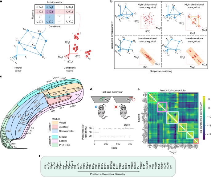
Data structure

We used the International Brain Laboratory (IBL) public data release⁴. For each experimental session, we collected time-series data on task, behaviour and electrophysiological recordings. These were segmented into trials based on key task events. The task recordings collected for each trial included information on the block prior as well as stimulus contrast and location. The behaviour recordings for each trial comprised the choice made, the outcome/reward received and the time-varying movement such as wheel movement velocity, whisker motion energy and licks. Other behavioural variables, such as paw movement, body motion energy and pupil diameter traces, could be potentially included. However, we did not include them because many sessions had missing values. The electrophysiological recordings for each trial contained time-varying spike trains of recorded neurons. All of these recordings can be accessed directly through the IBL’s open API. The following section describes the steps for preprocessing these raw data into data matrices for the encoding model.

Criteria for session inclusion

We iterated over all cortical regions and downloaded the related sessions. Sessions were included only if all of the behaviour recordings (wheel velocity, whisker motion energy and licks) and electrophysiological data were in place. A maximum of 30 sessions was included per cortical area to encourage a more balanced coverage. Some analyses required additional inclusion criteria, such as a minimum number of trials per condition. These analysis-specific criteria are discussed in the relevant sections below.

Criteria for trial inclusion

All trials from the left or right unbalanced blocks were included except when the animals did not respond to the stimulus in time (the first movement time was longer than 0.8 s). Trials from the 50–50 balanced block were excluded from the analysis to avoid possible time artifacts arising from the fact that all of these trials were exclusively recorded in the first 90 trials of the session.

Criteria for neuron inclusion

All neurons were included in the downloaded data provided that their mean firing rate was higher than 0.5 Hz and lower than 50 Hz. For the selectivity and geometry analyses, we included only neurons whose activity was predicted accurately enough by the RRR model described below (above a minimal threshold of \(\min \Delta R^2\) with respect to a simple model that assumes that the activity is equal to the average firing rate for all conditions). Unless specified differently, we used \(\min \Delta R^2=0.015\). This threshold was necessary to avoid confounding effects from neurons that do not encode any relevant variable, including those recorded with a low signal-to-noise ratio. Although the main results of our article remain qualitatively the same for a broad range of values of ΔR² (Extended Data Fig. 6), it is important to avoid the extreme cases (that is, when no neuron is discarded, or when too few neurons are selected) when studying whether the representations are categorical or not. Indeed, as already noticed previously¹³, when all neurons are considered, there is the risk that ‘junk’ neurons with very low selectivity to all variables are over-represented, leading to a peak in the distribution around zero selectivity. This distribution would be significantly different from our null distribution (multivariate Gaussian), but that does not mean the representation is actually categorical or that there is any interesting structure in the selectivity distribution. Indeed, in that previous study¹³, they used as a null distribution the superposition of two Gaussians: one representing the distribution of the selective neurons, and the other, peaked around zero selectivity, to describe the junk neurons. In our case, we decided to discard the worst neurons by selecting only cells that have a large enough ΔR². Again, the exact value is not important, but keeping all neurons would lead to an extra peak around zero selectivity, and a misleading, inflated number of brain areas that would pass the criterion for being considered categorical. Again, this is not a real, interesting structure and, in general, when performing this kind of analysis, we recommend checking that the structure revealed by a statistical test is not just due to the overrepresentation of junk neurons. Similarly, if only very few neurons are selected, the centre of the selectivity distribution might be depleted, leading again to the misleading conclusion that the representation is categorical.

RRR encoding model

In this section, we describe the RRR model used to analyse the selectivity profiles of single neurons. We start by describing the input and target variables of the model, followed by a description of the model itself and its fitting procedure. Finally, we introduce a few quantities resulting from the fitted model that are key to the follow-up analysis. The notation that will be used is summarized in the ‘Notations’ section. The code for implementing and fitting the encoding model is available at GitHub (https://github.com/realwsq/brainwide-RRR-encoding-model).

Input and target variables

Target variables

The target variables (y in equation (1)) were the preprocessed neuronal responses. The preprocessing steps were applied as follows:

1. 1.

   For each trial, we used the spike trains of the time window −0.2 to 0.8 s relative to stimulus onset, as the first movement time is typically less than 0.8 s (ref. ⁴). The activity of each neuron was first binned at 0.01 s, divided by the size of the time bin and then smoothed with a Gaussian filter with a s.d. of 0.02 s. We tried to apply the linear time warping technique⁵¹ so that the stimulus onset time and first movement or response time aligned across trials, but the results did not differ substantially.

2. 2.

   The resulting activity of neuron n, denoted as fr_n, was organized into a matrix of shape K_n × T, where K_n is the number of trials and T = 100 is the number of time steps per trial. K_n depends on n as neurons may have different numbers of trials if they were recorded in different sessions.

3. 3.

   Finally, for each neuron and each time step, we z-scored the activity fr across trials to obtain the target variable y as follows (Extended Data Fig. 1b,c,d):

   $$y_n(k,t)\,=\frac\mathrmfr_n(k,t)-\mu _n(t)\sigma _n(t),\,\mathrmwhere\,\mu _n(t)=\,\frac\sum _k\mathrmfr_n(k,t)K_n\,\mathrmand\,\sigma _n(t)=\,\sqrt{\frac\sum _k(\mathrmfr_n(k,t)-\mu _n(t))^2K_n}.$$

   (1)

   As the squared error between the preprocessed data and model predictions was used in the loss function for optimizing the model, the applied normalization prevented biases arising from inherent differences in activity scales and ensured that the predictions for all neurons and time steps were optimized equally. Notably, the z-score transformation is easily invertible, allowing the model’s predictions to be mapped back to the original units of firing rate, therefore preserving interpretability (Extended Data Fig. 1b–d).

Examples of the processed neural activity are shown in Extended Data Fig. 1b.

Input variables

The input variables (x; Extended Data Fig. 1a) that we considered can be divided into two types: discrete task-based variables and continuous movement variables. Discrete task-based variables include task-related features, such as the block prior, stimulus contrast, stimulus side, choice and outcome. These are listed below:

• Block: the prior probability for the stimulus to appear on the left side is either p(left) = 0.2 (right block) or p(left) = 0.8 (left block). We used one input variable to encode the block prior: −1. representing p(left) = 0.2, and +1. representing p(left) = 0.8. As noted above, we excluded trials from the p(left) = 0.5 unbiased block.

• Contrast: the stimulus contrast is 0%, 6.25%, 12.5%, 25% or 100%. One variable was used to encode the stimulus contrast: 0, representing 0% contrast; 1, representing the low contrast (≤12.5%); and 4, representing the high contrast (>12.5%).

• Stimulus: the stimulus location is either on the left side (+1) or the right side (−1).

• Choice: the choice is indicated by the turning of the wheel: clockwise (+1) or counterclockwise (−1).

• Outcome: the outcome is either a water reward (+1) or negative feedback (−1).

As these values are static, all of the timepoints share the same values (Extended Data Fig. 1a).

Continuous movement variables included both instructed (for example, licking and wheel velocity) and uninstructed (for example, whisker motion energy) movement. These were as follows:

• Wheel: the velocity of the wheel movement (radian per second) per time bin.

• Whisking: the whisker motion energy per time bin is calculated as the motion energy for a square of the left/right camera roughly covering the whisker pad. The maximum value between the left and right whisker motion energy was used.

• Lick: the number of licks per time bin.

A few preprocessing steps were applied separately to each movement variable:

1. (1)

   For each trial, we first read out the continuous behaviour of the time window −0.2 to 0.8 s relative to stimulus onset and interpolated into 0.01 s time bins.

2. (2)

   Then, to account for the activity that was shifted in time, for each session, we computed the mean time-lagged correlation between the neuronal activity and the movement traces averaged across neurons and trials and shifted the movement traces so that the zero-lagged correlation was maximized.

3. (3)

   Last, significant differences were observed in the variance of input values across trials, both for different input variables and different time steps. To ensure optimal performance and clarity in interpretation, we z-scored the values for each input variable and time step across trials in the same way as in equation (1). The reasoning behind this normalization step is twofold. From a performance perspective, as an extra regularization term was incorporated to penalize the high-value coefficients, the scales of the coefficients and, therefore, the scales of the input values should be comparable for the regularization to work properly. From an interpretability standpoint, the inherent differences in scales must be carefully addressed to enable the comparison of coefficients across input variables and time steps.

Examples of the resulting input variables are shown in Extended Data Fig. 1a.

The model formulation

Linear encoding model

For each neuron n, we describe its temporal responses as a linear, time-dependent combination of input variables (a visual illustration is shown in Fig. 2a and Extended Data Fig. 1):

where

• y_n(k,t) is the preprocessed neuronal activity of the trial k ∈ 1, …, K_n and time step t ∈ 1, …, T.

• \(\widehaty_n(k,t)\) is the corresponding model prediction, given by the value of the equation on the right side.

• v represents the relevant input variables included in the model. x^v(k,t) is the preprocessed value of the input variable v for the trial k and time step t.

• \(\beta _n^v(t)\) is the effect size of the input variable v at time step t. It is further referred to as the regression coefficient.

Low-rank coefficient matrix

The time-varying coefficients \(\boldsymbol\beta _n^v\in \rm\mathbbR^T\) are the weighted sum of a set of temporal basis vectors shared across all of the neurons and input variables, that is

Here, \(\bfU_n^v\in \rm\mathbbR^d\) is the neuron n and input variable v-dependent loading of temporal basis vectors \(\bfV\in \rm\mathbbR^d\times T\). Specifically, we considered sharing a single set of temporal basis vectors across all of the neurons from all of the brain regions and across all of the input variables. We verified that this restriction did not compromise the goodness-of-fit. The rank d is generally a value much smaller than the number of time steps T. See Extended Data Fig. 1e for an example decomposition. Sharing the temporal bases across neurons and input variables significantly reduces the number of parameters (Extended Data Fig. 1f). Let N be the number of neurons, T be the number of time steps and ∣v∣ be the number of input variables. An unconstrained full-rank coefficient matrix uses N × ∣v∣ × T parameters, while a reduced-rank coefficient matrix of the same shape only needs N × ∣v∣ × d + d × T parameters. As N and T are typically much larger than d, the reduction in parameters is on the order of T, that is, around 100-fold.

Comparison to previous regression models

Well-established linear encoding models include generalized linear model (GLM)^4,19 and kernel regression model²⁰. Below, we first describe these two models and then discuss how they compare to our RRR model. GLM is expressed as

where the input filter vector, \(\boldsymbol\beta _n^v\), composed of \(\beta _n^v(t\prime )\) over a neighbouring time window, is factorized as

Here, κ^v represents pre-specified temporal basis vectors, which are not trained. Adapted from a previous study⁴ (here we considered neural responses over a different time window from⁴ and an enriched set of behaviour movements), we used the same set of raised cosine ‘bump’ functions in log space for Extended Data Fig. 1h. The kernel regression model uses the same linear formulation as the GLM (equation (4)). However, instead of relying on pre-defined temporal basis vectors, it allows these vectors to be trainable:

Both the kernel regression model and our RRR model fall into the category of RRR models. The primary distinction lies in the set of input features used by each approach.

In our RRR model, the influence of input variables on neural responses, \(\beta _n^v(t)\) can vary over time. By contrast, both the GLM and the kernel regression model assume that the influence is time-independent. Therefore, for example, whether the mouse response time is early or late makes no difference and will modulate the neural responses the same way. Instead, these models provide a more descriptive account of input effects by allowing neural responses to depend on inputs from neighbouring time steps. While this feature is absent in our current RRR model (equation (2)), it could be incorporated in future extensions. A performance comparison is shown in Extended Data Fig. 1h.

Estimation of the parameters

The parameters of the RRR model include a shared temporal bases matrix V of size d × T and loading vectors \(\bfU_n^v\) of length d for each input variable v and neuron n. The approach we adopted to fit the parameters was to minimize the ridge-penalized mean square loss:

Minimizing this particular loss function is straightforward as a closed-form solution exists⁵². In practice, we chose to use the L-BFGS optimization algorithm to compute the optimum.

Moreover, to optimize the model hyperparameters, namely the rank d and the regularization penalty λ, we implemented a threefold cross-validation technique across trials. First, the dataset was stratified based on a composite target label that included the block prior and stimulus contrast to ensure that each fold was representative of the entire dataset. Then, for each combination of d and λ, the dataset was partitioned into three subsets by trials, using each subset in turn for testing the model while the remaining data served as the training set. Finally, the combination of d and λ that yielded the lowest average test error across all folds was selected. d = 5 turned out to be the optimal number of temporal bases.

Estimating the goodness of fit

We used the threefold cross-validated R² to measure the goodness-of-fit of single-trial predictions. For each session’s data, we randomly sampled one-third of the trials as the test set held out during training. Once the model was trained—using the remaining two-thirds of trials—we computed the R² between the model predictions \(\hat\mathrmfr_n(k,t)\) ((\(\hat\mathrmfr_n(k,t)\) is calculated by inversing the z-score transformation applied in the preprocessing step \(\hat\mathrmfr_n(k,t)=\sigma _n(t)\haty_n(k,t)+\mu _n(t)\); Extended Data Fig. 1b–d) and the actual neuronal activity fr_n(k,t) in the test set. We repeated the whole split–train–test process three times and computed the mean of the three cross-validated R² as the measure of goodness-of-fit.

Null model and selectively modulated neurons

Conceptually, we distinguish two types of task modulation: the selective modulation and the non-selective modulation. Selective modulation, captured by \(\haty_n(k,t)=\sum _v\beta _n^v(t)x^v(k,t)\) is induced by the input variables and varied trial by trial. Non-selective modulation, captured by the mean time-varying response \(\mu _n(t)=\frac\sum _k\mathrmfr_n(k,t)K_n\) is locked to the key events of the trial (stimulus onset in this case) and does not vary trial by trial. Both types have an important role in modulating neuronal responses. See Extended Data Fig. 2b for example selectively modulated (left) and non-selectively modulated (right) neurons. In this work, we focus mostly on the neuronal responses selectively modulated by the task. To distinguish the variation explained by the selective modulation from the non-selective modulation, we use the trial-average estimate as the null model that does not consider any effect of the input variables:

The outperformance, ΔR², defined as:

captures the overall selective modulation of all of the input variables combined.

Only selectively modulated neurons, identified as ΔR²(RRR) ≥ 0.015 (Extended Data Fig. 1g), are included in the further analysis.

Computing the selectivity profiles of single neurons to the input variable

To compute the selectivity profiles of single neurons to the individual variables, we used the estimated coefficient \(\beta _n^v(t)\). For the clustering analysis of Fig. 3 and Extended Data Fig. 6, we took the sum of the coefficients across time as a measure of the total selectivity of neuron n to input variable v.

Note that by normalizing the neuronal responses and input variables in the preprocessing steps, we ensured that the unit-free coefficients \(\beta _n^v(t)\) are not affected by the neuron’s mean firing rate or the inherently different scales in different input variables and can be compared directly across neurons, input variables and time steps. Thus, \(\beta _n^v(t)\) can be interpreted as the expected change in normalized neuronal activity y_n per one s.d. change in the input variable x^v at time t, and \(\alpha _n^v\) can therefore be thought as the expected total change across the whole trial.

The selectivity \(\alpha _n^v\) captures whether individual neurons are selectively modulated by the given variable v or not (examples of strongly selective neurons are shown in Extended Data Fig. 2c). In the selectivity analysis (Fig. 2e,f), when the goal is to estimate the absolute modulation of an input variable, \(\alpha _n^v\) is calculated as \(\alpha _n^v=\sum _t| \beta _n^v(t)| \).

Computing the autocorrelation timescale of neural responses to task and behaviour variables

Given a matrix of single-neuron responses to task and behaviour variables \(\haty_n\in \rm\mathbbR^K\times T\) with K being the number of trials and T the number of time steps per trial, we can compute the corresponding autocorrelation timescale.

To compute the timescale, we first calculate the time-lagged unnormalized autocorrelation sequence

We then linearly interpolate the autocorrelation sequence so that c_n(i) is spaced at 1 ms resolution (original 10 ms). The timescale τ_n is approximated by the time the sequence first reaches half its peak value (that is, c_n(0)). The timescale of brain area a is further determined by averaging the values over all of the selectively modulated neurons within this area.

We observed a significant correlation between a region’s hierarchical position and its estimated autocorrelation timescale (Extended Data Fig. 2d).

Notations

• Indices:

  • n, N: index and number of neurons (n ∈ 1, …, N).

  • k, K: index and number of trials (k ∈ 1, …, K).

  • t, T: index and number of time steps (t ∈ 1, …, T).

  • v, \(| v| \): index and number of input variables (v ∈ block prior, stimulus contrast, stimulus side, choice, outcome, wheel velocity, whisker motion energy, lick).

  • i, d : index and rank of the RRR model (i ∈ 1, …, d).

• RRR model

  • \(\beta _n^v(t)\): regression coefficient (arbitrary units (a.u.)) of neuron n, input variable v at time step t.

  • \(\bfU_n^v\in \mathbbR^d\): neuron n and input variable v-dependent loading of temporal basis vectors (a.u.).

  • \(\bfV\in \rm\mathbbR^d\times T\): temporal basis vectors (a.u.).

• Random variables:

  • x^v(k,t): preprocessed value (a.u.) of input variable v, trial k at time step t.

  • y_n(k,t): preprocessed neuronal response (a.u.) of neuron n, trial k at time step t.

  • \(\widehaty_n(k,t)\): model prediction of preprocessed neuronal response (a.u.) of neuron n, trial k at time step t.

  • fr_n(k, t): smoothed, binned firing rate (Hz) of neuron n, trial k at time step t.

  • \(\hat\mathrmfr_n(k,t)\): model prediction of smoothed, binned firing rate (Hz) of neuron n, trial k at time step t.

  • μ_n(t): mean of smoothed, binned firing rate (Hz) of neuron n at time step t.

  • σ_n(t): s.d. of smoothed, binned firing rate (Hz) of neuron n at time step t.

Clustering analysis

To test for the presence of functional clusters, we followed the steps explained below. The required inputs include each relevant neuron’s response profile and original session ID. Two types of response profile can be considered: the estimated selectivity to individual input variables (equation (10), referred to as clustering analysis in the variable selectivity space, used in Fig. 3 and Extended Data Fig. 6) or the average response in each experimental condition (referred to as clustering analysis in the conditions space, used in Extended Data Fig. 6). Performing clustering analysis in the selectivity space arguably has a few advantages: (1) It reduces the dimensionality in an interpretable and informed way. If we have ∣v∣ variables, then there are at least 2^∣v∣ conditions, assuming all of the variables are discrete and have more than one different value. (2) It mitigates the issue of unbalanced or even missing conditions. (3) It reduces the noise in the estimation of the response profile. As shown in Fig. 2b and Extended Data Fig. 2, neural responses are very noisy, and simple averaging may be non-satisfactory. By contrast, the selectivity estimated from the encoding model provides a more reliable account of the task-driven variance in the neural responses.

The code for the clustering analysis is available at GitHub (https://github.com/realwsq/clustering-analysis).

Clustering analysis in the variable selectivity space

We summarize our clustering pipeline as follows (a schematic is shown in Fig. 3a). (1) Check whether there are more than 50 neurons and only continue if so. (2) Given the selectivity profile of each neuron, run the k-means clustering algorithm (with 100 random initializations) with the number of clusters k varied from 3 to 20. (3) Then, select the optimal clustering result by maximizing the silhouette score. The silhouette score is defined as \( < \fracb_i-a_i\max (b_i,a_i) > _i\) where i is the index of the neuron, \(a_i=\frac1 -1\sum _j\in C_I,i\ne jd(i,j)\) is the mean Euclidean distance intracluster and \(b_i=\min _J\ne I\frac1\sum _j\in C_Jd(i,j)\) is the minimum Euclidean distance outside cluster (Fig. 3a). (4) Iterate over the resulting clusters and check whether there is a cluster whose total silhouette score summed over all neurons is mainly contributed by neurons from one single session (>90%). If so, remove neurons from that cluster and session, and repeat steps 1–4. (5) Sample the same number of datapoints from the Gaussian distribution with the mean and covariance matrix matched to the data values and compute the sampled data’s null silhouette score according to steps 2 and 3. (6) Repeat step 5 100 times and pool the null silhouette scores to form the null distribution. Finally, compute the z score of the data silhouette score with respect to the null distribution.

Clustering analysis in the conditions space

When clustering in the space of mean firing rate, two additional preprocessing steps are required. First, we normalized each neuron’s mean firing rates separately across conditions to prevent clustering driven solely by overall firing rate differences between neurons. Second, as the number of conditions and the dimensionality of the activity profile is high, we reduced the dimensionality using principal component analysis. Moreover, we modified the null model by replacing the multivariate Gaussian distribution with a multivariate log-normal distribution to better capture the lower-bounded and heavy-tailed nature of mean firing rates. Neurons with zero activity were excluded from this analysis.

The clustering analysis in the conditions space follows these steps (a schematic is shown in Extended Data Fig. 5): (1) check whether there are more than 40 neurons and only continue if so. (2) z-Score the mean firing rates for each neuron. (3) Reduce the dimensionality using principal component analysis, retaining components that capture 90% of the total variance. (4) Run the k-means clustering algorithm (with 100 random initializations), varying the number of clusters k from 3 to 20. (5) Select the optimal clustering result by maximizing the silhouette score. (6) Iterate over the resulting clusters and check whether there is a cluster whose total silhouette score summed over all neurons is mainly contributed by neurons from one single session (>90%). If so, remove neurons from that cluster and session, and repeat steps 1–5. (7) Sample the same number of datapoints from the multivariate log-normal distribution with the mean and covariance matrix matched to the log data values, then compute the sampled data’s null silhouette score following steps 2–5. (8) Repeat step 7 100 times and pool the null silhouette scores to form the null distribution. Finally, compute the z score of the data silhouette score with respect to the null distribution.

Measuring the similarity between cluster and area labels

The similarity between functional clusters and anatomical area labels was quantified using the RI, which measures the agreement between two labellings of the same dataset. For each pair of neurons, agreement occurs if both are assigned to the same cluster in both labellings, or to different clusters in both. The RI is defined as the fraction of agreeing pairs among all possible pairs. To assess statistical significance, we computed a z-scored RI by comparing the observed RI to a null distribution obtained from 10,000 random shufflings of the area labels. A significantly elevated z-scored RI indicates that functional clustering aligns closely with anatomical organization. To avoid biases towards areas or modules with larger neuron numbers, we considered the 100 best-encoded neurons from each module or area in the analysis of Fig. 3e,f and Extended Data Fig. 7.

Modified ePAIRS test

Given the average responses of single neurons in each experimental condition, we performed the ePAIRS test as follows (a schematic is shown in Extended Data Fig. 5): (1) z-score the mean firing rates for each neuron. (2) Reduce the dimensionality using principal component analysis, retaining components that capture 90% of the total variance. (3) Calculate the cosine distance to its nearest neighbour for each neuron. (4) Calculate the empirical median of these nearest-neighbour distances as the aggregated nearest-neighbour angle. (5) Sample the same number of datapoints from the multivariate log-normal distribution with the mean and covariance matrix matched to the log data values, then compute the null nearest-neighbour angle of the sampled data according to steps 1–4. (6) Repeat step 5 5,000 times and pool the null nearest-neighbour angles to form the null distribution. Finally, the z-score of the data aggregated nearest-neighbour angle with respect to the null distribution is computed.

α-Diversity

To measure α-diversity, we took the participation ratio of the N × V matrix of α coefficients resulting from the RRR analysis described above. The PR quantifies the effective dimensionality of a set of datapoints by measuring how evenly the variance is distributed across the eigenvalues of its principal component analysis decomposition²⁸. The PR is defined as:

where λ_j is the jth eigenvalue of the N × N covariance matrix. A higher PR indicates that the variance is more evenly spread across multiple dimensions, suggesting a higher effective dimensionality of the cloud of points in the high-dimensional space. Conversely, a lower PR implies that the variance is concentrated in fewer dimensions, indicating a lower effective dimensionality.

The number of neurons in individual areas was soft-equalized by taking a random subsample of N₀ = 120 neurons when N > N₀. In these cases, the participation ratio was computed over 100 random subsets, and the average was taken as the value of α-diversity.

Analysis of population representations

Data preparation

For the analysis of population neural representations, we used the same sessions as described above. For each trial within a session, we therefore have a collection of N-dimensional population activity vectors f^t,k, where k ∈ 1, P is the trial index within the session, and t ∈ 1, T is the time-bin index within each trial. For the analysis below, we used data from 0 to 1,000 ms after the stimulus onset to capture a variety of sensory and behavioural variables. We then labelled each time bin according to the value of four binarized cognitive, sensory and movement variables:

• Block: left (20–80) versus right (80–20) prior block.

• Contrast: we binarized the contrast into low (0–0.125) versus high (0.25–1.0) values.

• Stimulus: left versus right side of the screen.

• Whisking: we binarized the whisking power using the distribution of whisking power values within each session. Time bins in which the mouse was whisking with a power larger than the 50th percentile across the distribution were annotated as high, while those below the 50th percentile were annotated as low.

These variables were chosen so that they span movement, cognitive and sensory variables while ensuring that all of the M = 16 conditions (combinations of the four variables) were well represented in the data. For example, we could not add Choice as a variable as mice are overtrained in the task and, as a consequence, make very few mistakes when block and stimulus are aligned (for example, choose ‘left’ when the block and the stimulus are both ‘right’).

For each condition c ∈ 1, M (for example, whisking = high, contrast = low, stimulus = left, block = right), we first identified those trials in which that specific combination of variables was present. We then defined a collection of ‘conditioned trial’ population activity vectors f^k,c as the mean firing rate of the population of neurons conditioned to the specific condition in each trial. Given a trial k and a neuron index i, the mean firing rate was computed as

where i indicates the neuron index and δ^t,k(c) = 1 if the time bin t in trial k corresponds to the condition c, and 0 otherwise. These conditioned trial population vectors are the data samples that will be used for the dimensionality and decoding analyses below. Across all analyses, we considered only those recording sessions in which each condition was present in at least M_min = 5 trials.

Representation dimensionality

To estimate the representation dimensionality of a neural geometry, we computed the PR of the centroids f_c of the M conditions, defined as the average activity pattern across all trials of the same condition:

To compute the PR for the set of centroids, we first calculated their covariance matrix, normalizing each neuron’s mean activity vector by subtracting from each \(f_i^c\) the mean across conditions c and dividing them by their s.d. We then performed principal component analysis on this covariance matrix to obtain its eigenvalues, λ_j.

The number of neurons in individual areas was soft-equalized by taking a random subsample of N₀ = 120 neurons when N > N₀. In these cases, the participation ratio was computed over 100 random subsets, and the average was taken as the value of representation dimensionality. The PR was computed on the set of centroids to highlight signal dimensions and prevent noise from dominating the measure. When computed across all trial vectors (without condition averaging), the PR ranged from 10 to 350 and was highly correlated with that of the centroids (Spearman Correlation coefficient = 0.86).

Cross-validated decoding

We used Decodanda⁵³ (www.github.com/lposani/decodanda) to perform a cross-validated, class-balanced decoding analysis of different combination of condition labels from the neural activity within individual trials (condition trial vectors f^k,c). See the individual sections below for additional details on the data input structure of our decoding analyses. As a decoder, we used a scikit-learn SVM classifier with linear kernel⁵⁴. To ensure that results were comparable across regions, which might have a different number of recorded neurons, we created a pseudopopulation by resampling all of the recorded neurons within each region to a fixed number N = 4,000. Similarly, we resampled the same number of pseudopopulation for each analysis (T = 100 patterns per condition). Note that simultaneously recorded neurons were always kept together during resampling to keep the noise correlations intact within the pseudopopulation⁵³. All cross-validated decoding analyses were performed using the following Decodanda parameters: training_fraction = 0.8, cross_validations = 100, ndata = 100.

Finding the independent conditions

To find the number of independent conditions encoded in the activity of a population of neurons, we developed an iterative algorithm based on linear decoding. The algorithm followed the steps below, and is shown in action on one example region in Extended Data Fig. 3.

1. (1)

   First, we performed a decoding analysis of the condition label c from trial population vectors f^k,c using a set of binary linear classifiers. For each pair of conditions (c_i, c_j), we estimated a cross-validated decoding performance φ(c_i, c_j), resulting in an initial M × M condition–condition decoding matrix (C₀; Extended Data Fig. 3) defined as C₀(ij) = φ(c_i, c_j).

2. (2)

   We then chose a decoding threshold \(\varphi _\min =0.666\); the pairs of conditions whose one-versus-one decoding performance was smaller than \(\varphi _\min \) were defined as dependent. Using this threshold, we defined a binary dependency matrix D defined as D₀(i, j) = 1 if \(\varphi (c_i,c_j) < \varphi _\min \), and C₀(i, j) = 0 otherwise.

3. (3)

   We then used the Bron–Kerbosch algorithm⁵⁵ to find all of the cliques, that is, subgroups of fully connected nodes, in the undirected graph defined by the dependency matrix D₀. This process enables us to identify whether there are groups of conditions that are all non-decodable from each other (dark squares in the sorted matrix in Extended Data Fig. 3).

4. (4)

   We next identified the largest clique and grouped together all of the trials of the conditions within that group into a new, merged condition (see the arrows and ‘merge’ conditions in Extended Data Fig. 3).

5. (5)

   We repeated steps 1 and 2 with the new reduced set of conditions, yielding a new C_t and a new D_t matrix of a different size M_t, where t denotes the iteration step.

6. (6)

   We then repeated steps 3 and 4, and iterated the whole process (1–4) until all of the merged and remaining conditions were found to be independent, that is, the dependency matrix \(D_\widetildet\) was diagonal. The number of independent conditions was then defined as the size of the final dependency matrix: \(M_\mathrmIC:=M_\widetildet\).

Separability and AD

Separability quantifies how many random dichotomies (equally sized groups) of experimental conditions can be decoded from neural activity using cross-validated linear classifiers. To estimate the separability of a neural population, we performed the following steps:

1. 1.

   First, we randomly divided the set of M or M_IC independent conditions into two equally sized groups (dichotomy).

2. 2.

   Given the dichotomy d, we then measured the cross-validated decoding performance φ_d of a linear classifier trained to report whether individual condition trial vectors f^k,c belonged to conditions within one or the other dichotomy groups. This decoding analysis was performed as described in the ‘Cross-validated decoding’ section above, resampling a fixed large number of neurons (N = 4,000) and a fixed number of trials (T = 100) per condition for all regions to ensure that performances could be compared across regions.

3. 3.

   The random dichotomy assignment and decoding (steps 1 and 2) was then repeated n = 200 times to obtain a set of decoding performances φ_d.

4. 4.

   The decoding analysis was then repeated n = 200 times with shuffled condition labels across the population vectors to obtain a distribution of null decoding performance values φ^null.

5. 5.

   Separability was then defined as the fraction of decodable dichotomies, that is, the fraction of φ_d larger than the 99 percentile of the null population φ^null. AD was defined as the mean decoding performance across the n = 200 random dichotomies.

The distributions of decoding performances for all of the analysed regions are shown in Extended Data Fig. 11.

Synthetic data

Modelling uneven and categorical selectivity

We generated synthetic population responses for N neurons to all 2^V configurations of V binary variables x_v ∈  − 1, 1. Each neuron’s response combined linear and quadratic selectivity,

where γ controls the strength of non-linear interactions and \(\epsilon _i \sim \mathcalN(0,\sigma )\) introduces trial-to-trial variability. For each condition \(\vecx\), we generated T independent trials and used the data in the decoding analyses as performed for real spiking data.

Sampling the selectivity structure

The coefficients (α_iv, β_i,uv) were sampled in a feature space of dimension \(D=V+\fracV(V-1)2\), which groups all linear and quadratic features on an equal footing. To generate either categorical or uneven selectivity, we first drew k cluster centroids in the D-dimensional feature space and repeated each centroid k_N = N/k times, yielding N prototype vectors. These prototypes define the coarse structure of selectivity across neurons. To modulate within-cluster diversity, each prototype was perturbed by an additive diversity vector

where \(\sigma _d=-\log (c)\) is set by a categorical specialization parameter c ∈ (0, 1) (this is the x axis in Extended Data Fig. 8b). Larger c produces more tightly clustered selectivity (strong categorical structure), whereas smaller c yields more dispersed coefficients. To model uneven selectivity, we introduced anisotropy across the D feature dimensions by using k = 1 (no clustering) and scaling the diversity terms by a geometric decay profile:

where r ∈ (0, 1) is the global specialization parameter. When r ≪ 1, all dimensions contribute equally; when r ≈ 1, variance is concentrated in a low-dimensional subspace, producing a strongly uneven selectivity spectrum. The final coefficients, including categorical and/or uneven structure, were

with the quadratic coefficients additionally scaled by γ to control non-linearity.

Trial generation

For each of the 2^V binary stimuli, we computed \(f_i(\vecx)\) through the linear-quadratic form above, and generated T noisy samples per condition,

This procedure ensures that trial variability is independent across neurons and conditions, and that all structure in the population code arises exclusively from the geometry of the sampled coefficients.

Parameterizing categorical and uneven specialization

The two specialization parameters (c, r) therefore independently control: the categorical structure of selectivity (the number and separation of clusters, through c and k); and the unevenness of selectivity across feature dimensions (anisotropy of coefficient variances, through r).

By sweeping either c (categorical specialization) or r (global specialization) while keeping the other fixed, we isolated the effects of clustered versus uneven selectivity on representational dimensionality, separability and independent condition structure. For the analyses in Extended Data Fig. 8, we used N = 100 neurons, V = 3 variables (for a total of P = 8 conditions), T = 20 samples per condition and γ = 0.25.

Exploring the relationship between dimensionality and separability

To analyse how separability changes with the dimensionality of the geometry in the activity space, we performed a series of synthetic explorations shown in Extended Data Fig. 8. In these simulations, P centroids are randomly sampled from a Gaussian distribution spanning an L-dimensional subspace of the N-dimensional activity space. Each centroid vector is normalized. Trial-to-trial variability is then added to the centroids with a s.d. σ, scaled with \(\sqrtL\) to keep the signal-to-noise level constant when pairwise distances between centroids increase with L. This obtains a T × N activity matrix for each of the P conditions. This synthetic activity is then analysed with the same pipeline used for the cortical data, yielding values of representation dimensionality, separability and AD shown in Extended Data Fig. 8g, in which we used P = 16, N = 100. For simulations in Extended Data Fig. 8i, we fixed L = 14 and multiplied the first dimension of each centroid by a factor γ to stretch the geometry along a single axis.

Theoretical considerations on the relationship between dimensionality and clustering

The conditions space and the neural space have the same dimensionality

As explained in Fig. 1a, response profiles of single neurons can be thought of as rows of a matrix X for which the columns define the geometry of conditions in the neural space. The PR in the conditions space is computed from the eigenvalue spectrum of the covariance matrix of the rows of X, that is, XX^T (assuming zero mean), while the PR in the activity space is computed from the eigenvalues of the covariance matrix of the columns of X, that is, X^TX. Given a matrix, the eigenvalues of its covariance matrix are the squared singular values of X. Let X = USV^T be the SVD decomposition of X, where S is the diagonal matrix with singular values on the diagonal, then X^T = VS^TU^T. As S = S^T, the eigenvalue spectrum of X^TX and XX^T is the same. Thus, the participation ratio of the conditions space is the same as that in the neural space.

Mathematical derivation of the PR of Gaussian clusters

We consider a data model with N features (neurons) and M observations (conditions), in which observations are sampled from independent and identically distributed (i.i.d.) random variables as

where z^μ and η^μ are both vectors in \(\mathbbR^N\) and represent the clustered and heterogeneous part of the data, respectively. More precisely, z^μ is sampled from a normal distribution \(\mathcalN(0,\bfB)\) that has a clustered covariance matrix, that is, B_ij = 1 if i and j belong to the same cluster and B_ij = 0 otherwise. We call k the number of clusters and assume that all clusters have the same number of neurons N_c = N/k. By contrast, the heterogenous part η^μ is sampled from \(\mathcalN(0,\sigma ^2\bfI)\), where I is the identity matrix. Our goal is to compute the participation ratio (PR) of this representation, which we define as

where the averages are across neurons and the matrix C is the sample neuron-by-neuron covariance matrix, that is \(C=\frac1M\sum _\mu =1^M\bfx^\mu (\bfx^\mu )^T\). We note that this definition assumes that the sample mean of both z and η are negligible or have been subtracted.

We are interested in the regime in which N → ∞ while M is allowed to be small, as it often happens in controlled experiments. Small M might cause the sample covariance matrix to differ substantially from the true covariance matrix. Defining C^c, C^h, and C^ch as the sample covariance matrices of z, η, and the cross-covariance between z and η, respectively, we have that

We therefore need to evaluate the first and second moments of both diagonal and off-diagonal elements of all covariance and cross-covariance matrices. The diagonal elements of these matrices have the following statistics:

and

For the off-diagonal elements, we have

and

Most of the expressions above can be straightforwardly derived by writing down the definition of the sample covariance matrix for a zero-mean variable and then performing the average over neurons. To illustrate this procedure, let us consider one of the most involved terms:

The probability that z_i and z_j are part of the same cluster is given, for large N, by \(\frac1k\). The expression for \(\langle (C_ij^c)^2\rangle \) then becomes

The other terms can be computed following the same steps.

Given that k, M are finite, we can approximate the PR for large N as:

Expanding the square and using the results above for the first and second moments of the covariance matrices, we get to our final expression:

From the mathematical expression in equation (25), we can see that, in the limit of perfect clusters (σ → 0), the function is either limited by the number of rows-neurons (in this case, the k perfect clusters) or columns-conditions M, coherently with the intuition above:

However, things become more nuanced when k, M and σ are finite and non-zero. First, as shown in Fig. 5e, when k and M are kept fixed, the representation dimensionality decreases with the clustering quality (expressed as the average silhouette score of a population of Gaussian clusters with given k, M and σ). Second, if we fix the quality of clusters and the number of conditions (Fig. 5e (left)), we see that dimensionality increases with the number of clusters, with a magnitude that is larger for high silhouette scores (categorical representations). Finally, when fixing the number and quality of clusters, the dimensionality is determined by the number of conditions, with a magnitude that is larger for low silhouette scores (non-categorical representations; Fig. 5e (right)).

Different measures of dimensionality

Measuring dimensionality in the presence of noise and determining whether it is high or low can be quite challenging⁷. This is why, in neuroscience, multiple methods are used to assess dimensionality. Each approach is different and, as dimensionality is expressed as a single number, it inevitably emphasizes only specific aspects of the representational geometry.

In our Article, we always refer to the embedding dimensionality of the set of points representing different experimental conditions in the activity space⁵⁶. These points represent patterns of activity recorded at the same time (not trajectories). To discount the dimensions due to the noise, we computed the representation dimensionality of the average positions of the conditions. An alternative approach is to consider a cross-validated measure of representation dimensionality⁵⁷. Notice that separability and other measures related to it⁶, which consider the computational consequences of high dimensionality, are typically insensitive to noise, as they are also cross-validated measures.

Other recent works have introduced dimensionality measures that depend on the spatial and temporal scales considered⁵⁸. For large scales, they get an estimate of the embedding dimensionality and, for short scales, they get an estimate of the intrinsic dimensionality. While these quantities can reveal many other interesting aspects of the representational geometry, here we focused only on the embedding dimensionality because it is the one most relevant to the performance of a linear readout.

Reporting summary

Further information on research design is available in the Nature Portfolio Reporting Summary linked to this article.