A direct black-hole mass measurement in a little red dot at high redshift

Conventions

Throughout this work we assume a flat Λ (dark energy) cold-dark-matter cosmology with matter density parameter Ω_m = 0.315 and a Hubble constant H₀ = 67.4 km s⁻¹ Mpc⁻¹ (ref. ⁴⁶). All reported magnitudes are in the AB system. Following the lensing model of ref. ¹³, we adopt a flux magnification factor μ = 6.2 and a shear factor of 3.52 for our source (image A of QSO1). Hence, 1 arcsec in the image plane corresponds to 1.52 physical kiloparsecs. For robustness tests, we use the Bayesian information criterion (BIC), defined as BIC ≡ χ² + klnn, where k is the total number of model parameters and n is the number of points fitted; a decrease in BIC, ΔBIC ≥ 5, between two models was required for robust preference of one over the other, although our main conclusions remain unchanged even if a stricter ΔBIC ≥ 10 threshold is adopted.

Data reduction

We use data from the BlackTHUNDER NIRSpec integral field unit survey, focusing on the 7.3-hour exposures with the G395H grating, giving a nominal spectral resolution R = 3,700 at the wavelength of Hα¹⁵. The NIRSpec integral field unit was centred on image A of QSO1 (right ascension 00:14:19.161; declination −30:24:05.664)¹². A detailed description of the reduction procedures is available in refs. ^4,15; however, a summary is provided here for context.

The spectra were extracted following the procedures of ref. ⁴⁷, but using version 1.17.1 of the JWST pipeline. At z = 7.04, the Hα line falls just outside the nominal wavelength coverage; however, the F290LP filter does not cut off longer wavelengths and the detector efficiency allows to recover Hα emission. We perform this recovery by extrapolating the wavelength solution, flat-field curves and the grating-equation-derived line spread function (LSF) out of the nominal range and towards the detector sensitivity limit of λ = 5.34 μm. The peak of the Hα line of QSO1 falls on λ = 5.278 μm; hence, our modification readily recovers the entirety of Hα emission. Although flux calibrations beyond the nominal range may suffer inaccuracies, the primary interest of this work is a kinematics study; hence, our key kinematics results are insensitive to flux calibrations. The BH mass measurements are more affected. However, the square-root dependence of the BH mass on luminosity means that flux calibrations have to be wrong by an order of magnitude to significantly impact the measurements.

The nominal spaxel scale of the processed data was 0.05″; however, utilizing the large number of dithers, we are able to oversample the cube to a scale of 0.02″ per spaxel without incurring significant sampling artefacts. We choose the 0.02″ cube for the main kinematic and spectroastrometric analysis, with the 0.05″ cube used to perform consistency checks, ensuring that our results are not pixel sampling artefacts.

Spectroastrometry of the rotation curve

To constrain the density profile of QSO1, we combine spectroastrometric measurements with resolved kinematics. The technical details of spaxe-by-spaxel fitting and spectroastrometry are given in Supplementary Information sections 1.1 and 1.2; here we summarize that we subtract the broad Hα emission from the cube and create images of different velocity channels of narrow Hα for which centroids can be obtained at sub-point-spread-function scales (provided a sufficient signal to noise⁴⁸) and used to map dynamics below the nominal instrumental resolution^49,50. The fiducial spectroastrometric analysis utilizing two velocity channels for higher signal to noise is shown in Extended Data Fig. 1. However, as shown in Fig. 2, splitting the line into finer bins does not change our results.

We infer the outer parts of the rotation curve by binning the line-of-sight velocity field (shown in Fig. 1) on scales >60 pc to avoid beam smearing. This procedure resulted in 4 bins covering the negative and positive sides of the rotation curve with ⟨vsini⟩ ≈ 10 km s⁻¹ (where v is the line-of-sight velocity and i is the inclination angle) with nominal uncertainties of order 1 km s⁻¹. However, these uncertainties, estimated through the standard root mean square (rms) weighting scheme, do not take into account the velocity field cross-correlation between spaxels of each bin owing to beam smearing and hence are probably significantly underestimated. An a priori derivation of the covariance matrix is intractable as it would require fitting individual dithers, which have far too low signal to noise. We thus use an empirical approach—scaling the naive rms-derived errors until the optimal model in the family of models fitted has \({\chi }_{{\rm{R}}}^{2}=1\). This yields an upper limit on the possible errors as it assumes that the optimal model is the ground truth. Consequently, using this method, we can establish a lower limit on the significance of the optimal model (which turns out to be a point mass) over other models considered.

For the spectroastrometric data points, we use a flux weighted average of the velocity channels, giving ⟨vsini⟩ = 51 ± 4 km s⁻¹. The factor of sini is written to explicitly state that these are the projected values, uncorrected for inclination.

As the resultant rotation curve, shown in Fig. 2, is sparsely sampled, we consider only simple one- or two-parameter models for fitting. Model curves were constructed following a Keplerian prescription:

where G is the gravitational constant, R is the distance from the centre and M(<R) is the mass enclosed within R. Our fiducial fit follows a point-mass assumption with M(<R) ≡ M ≡ constant , which yields log(M/M_⊙) = 6.75 ± 0.05. We note that the uncertainty on this value is purely a fitting error and could be underestimated; hence, we re-estimate the error using bootstrap resampling, taking into account the width of the velocity bins, and we estimate a more conservative measurement error of 0.15 dex.

To fit the curve with a compact stellar-mass distribution, we fit the data with an NSC model derived for the Milky Way by ref. ¹⁹ who find a density profile following an R⁻² power law in the central 5 pc and dropping off as R⁻³. From this density profile, we construct the following function for M(<R):

where A is the parameter setting the overall normalization and R_c is the radius at which the switch in the power-law profile occurs. It is important to note that this is different from the ‘effective radius’ R_e of the two-dimensional light distribution; in the case of the Milky Way NSC, the R_e is a factor of 0.84 smaller than R_c. We initially fit the NSC model fixing R_c to 5 pc, the same value as found by ref. ¹⁹. This fit is shown as a dashed grey line in Fig. 2 and produces a considerably worse \({\chi }_{{\rm{R}}}^{2}=3.2\) than the point-mass (pure BH) fit with \({\chi }_{{\rm{R}}}^{2}=1.0\). This corresponds to a difference in the BIC of about 11, indicating robust preference for the point-mass fit, particularly as our error rescaling procedure provides a lower limit on the significance of the preferred model. If R_c is allowed to vary freely, then the NSC best-fit model gives R_c = 10⁻⁴ pc with M(<R_c) ≈ 10⁶ M_⊙, which would imply extreme stellar densities, in excess of 10¹⁷ M_⊙ pc⁻³. Such densities are orders of magnitude above the densest stellar systems seen in the Universe and show that our NSC model effectively collapses to a point mass if R_c is not fixed. We estimate an upper limit on R_c by fitting a fixed value and lowering it until the difference in BIC between the best-fit and the fixed R_c model reduces below 5. This way we estimate R_c < 0.2 pc with M(<R_c) ≈ 10^6.2 M_⊙; this limit is over 1 dex below even the most compact NSC in this mass range in the local Universe⁵¹, as well as the dense star clusters found in the lensed Cosmic Gems arc by ref. ⁵², as illustrated in Extended Data Fig. 2. The upper limit on the NSC stellar mass is even lower if one adopts the density profile inferred for NSCs in other galaxies (ρ ∝ r⁻²)⁵³. Hence, a point mass is needed to account for our observed dynamics.

In addition to the NSC model described above we consider the Plummer sphere²⁰ model, frequently used to describe the density profiles of globular clusters. The enclosed mass function for the Plummer sphere takes the following form:

where M₀ is the total mass of the system and R_P is the scale radius. Although this model performs similarly well to the point mass, it does so by fitting R_P ≈ 10⁻⁴ pc and thus results in similar unphysically high stellar densities, as in the case of the NSC.

In addition to being excluded by the ΔBIC value, a Milky Way NSC-like density profile with R_c ≈ 5 pc produces a total stellar mass of 10^7.2 M_⊙, which is above constraints on the stellar mass derived from ultraviolet and optical emission as discussed in Supplementary Information section 1.8.

A remaining potential caveat of our analysis is that only isotropic velocity distributions were considered—velocity anisotropies could steepen the radial velocity gradient of a diffuse mass component⁵⁴, increasing the allowable extended mass. However, the steepness of the observed velocity gradient is such that any extended component collapses to a point when the scale radius is left free. Hence, it is unlikely that anisotropies of the underlying velocity field significantly skew our results.

Lastly, we explore what, if any, constraints on the dark-matter halo surrounding the object can be obtained from our data. We thus fit the widely adopted Navarro–Frenk–White density profile⁵⁵. The enclosed mass for which is given by:

where ρ₀ and R_s are the characteristic density and scale radius, respectively. However, as with the previous extended mass distributions, the above model collapses to a point with R_s ≈ 10⁻⁴ and ρ₀ ≈ 10¹⁴ M_⊙ pc⁻³, once more collapsing to a point mass and producing unrealistic densities. However, this does not imply that QSO1 resides outside of a dark-matter halo. Instead, our attempts at reproducing the kinematics with an extended density profile imply that any extended mass component is sub-dominant at the <200 pc scales probed by our measurements. We attempt the above analysis using Hβ narrow or [O iii]. However, these lines are too faint for constraining measurements.

MOKA3D kinematics modelling

The measurements described above, although self-consistent, do not fully take into account instrumental effects such as point-spread-function beam smearing and the emissivity distribution of the light tracers. In the simplified analysis above, we overcome these issues by leveraging spectroastrometry. However, to check the robustness of our conclusions if such effects are accounted for, we independently refit the narrow-line cube with the MOKA3D framework^21,22. MOKA3D is a 3D kinematic framework that can model conical outflows or disks by assuming spherical, conical or cylindrical geometries respectively, with any irregular distribution of the emitting clouds within the velocity field. The 3D model is populated with a distribution of fictitious clouds that account for the observed emission. These clouds are weighted according to the observed narrow Hα flux in each spaxel and spectral channel of the data cube. As described in the following, the model clouds follow an analytical velocity field as a function of the radius, whose parameters are fitted to reproduce the observed emission and kinematic features via least-squares minimization.

As in the previous analysis, we consider three potential mass distributions—a point mass, an NSC density profile and a Plummer sphere. For each potential mass distribution, we parameterized the model clouds’ circular velocity following equations (1)–(3). The free parameters of each kinematic profile are listed in Extended Data Table 1, specifically: total mass (in the case of the Keplerian rotation, this is the point mass); parameter A from equation (2), which represents the overall normalization of the NSC model; inclination of the disk (0° would be a face-on disk) or inclination of the outflow axis (0° outflow pointing towards the observer); effective radius of the density distribution (defined by equations (3) and (2) for the Plummer sphere and NSC models, respectively); intrinsic velocity for the outflow model; and the position angle of the kinematic configuration on the plane of the sky (measured clockwise from the top of the image). As discussed in ref. ²¹, to remove the degeneracies that are present when deriving 3D structures from the observed two-dimensional projections on sky, we minimized the numbers of free parameters by considering pure circular motions with no radial flows (except when testing the outflow scenario). For each potential mass distribution, we allowed the free parameters to vary in a wide range with no a priori constraints. Then, we ran the fitting routine—creating a 3D model cube with the same spatial and spectral binning as the observed data for each set of parameters. We then extracted the integrated model spectrum and compared with the observed one. The optimal set of parameters for each model was derived following the least-squares method of minimizing the distance between the observed and the model data cubes. During this procedure, we convolve the model cube with the point spread function and weight each fictitious cloud in the 3D model cube by the observed flux in each spectral channel of each pixel to ensure that any mismatch between model and data is solely due to assumptions on the underlying geometry and kinematics. This procedure allows us to obtain a 3D model cube—identical to the observed one in terms of spatial and spectral binning—from which we can compute moment maps to be compared with observations. In-depth descriptions of the principles being MOKA3D are provided in refs. ^21,22.

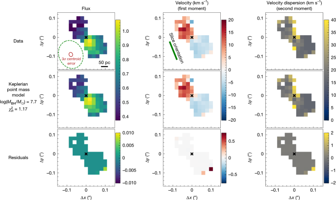
The comparison between the residuals of the different models is given in Fig. 1 (for the point-mass case) and Extended Data Fig. 3 (for the NSC and for the Plummer sphere cases). As can be seen in the figures, a point-mass profile is strongly preferred over any extended density profile. The Plummer sphere model, while leaving similar residuals to a Keplerian curve, does so with a scale radius \({R}_{{\rm{P}}}={0}_{-0}^{+3}\,\text{pc}\) (Extended Data Fig. 3), essentially collapsing into a BH. The NSC model remains extended even when R_c is allowed to vary (best-fit R_c = 4 ± 2 pc). However, it leaves significant systematic residuals in both velocity and velocity dispersion profiles, as shown in Extended Data Fig. 3.

As discussed in the following, very little velocity dispersion is included in the modelling (less than 7 km s⁻¹, well below the instrumental resolution) as the velocity dispersion in each pixel can be very simply reproduced by correctly modelling the line profile in each spaxel and weighting the model clouds against the observed flux; in other words, the apparent velocity dispersion is mostly and fully recovered simply by the velocity field, beam smearing and brightness distribution. In particular, a precise determination of the best-fit parameters via MOKA3D, combined with the innovative flux-weighting technique exploited by this model, guarantee to reproduce the observed moment maps at unprecedented detail, as demonstrated by refs. ^56,57,58. Indeed, by definition, moment maps are computed taking into account the flux distribution along the velocity space, which is what makes MOKA3D so effective in reproducing them once the observed and model line profile match. The crucial step of assigning the observed flux in each spectral and spatial channel to the corresponding model clouds that belong to the same channel is what allows MOKA3D to reproduce the observed feature with such high accuracy, once the model parameters are correctly inferred. It is important to stress that no flux distribution is ever assumed by MOKA3D but instead is recovered from the data via the weighting procedure and after the correct set of parameters is unveiled. This allows MOKA3D to reproduce extremely irregular and asymmetric features. Therefore, despite the set of best-fit parameters inferred with MOKA3D, any extended density profile is not the preferred parameterization to reproduce the observed features in each spaxel due to absence of model clouds with the necessary projected velocity.

To further clarify that the underlying MOKA3D kinematical model does not intrinsically have asymmetries, Extended Data Fig. 4 shows the intrinsic unweighted kinematical model underlying the full weighted model reported in Fig. 1. The asymmetric flux distribution (in the flux map) and asymmetric kinematic features (for example, in the velocity dispersion map) seen in Fig. 1 emerge only when MOKA3D weights each emitting clouds to optimally reproduce the observed (irregular) flux distribution.

It is notable that the MOKA3D point-mass model gives log(M_BH/M_⊙) = 7.7 ± 0.3 with an inclination of 52° ± 2°, entirely consistent with the lower limit obtained from the previous direct measurements. In fact, the spectroastrometric mass estimate, when corrected for the inclination becomes consistent with the MOKA3D value to within 2σ (6.9–7.2 versus 7.7 ± 0.3).

To test whether the inclination estimate is robust, as well as to verify the presence of a rotating disk, we construct a non-parametric model wherein the disk is split up into three distinct shells that are fitted with independent inclinations. We find that this model fits the data well and produces shell inclinations of approximately 45 ± 10°, consistent with each other and the value found by the parametric models (Extended Data Fig. 5). The fact that consistent results are obtained regardless of the precise analytical procedure used indicates that our measurements are robust. In Supplementary Information sections 1.4 and 1.5, we further consider, and rule out, contributions of outflows to the narrow-line kinematics.

We also note that a diffuse, extended (exponential) disk-like mass distribution (M ≈ 10⁷ M_⊙, R_s = 150 pc), while reproducing the large-scale (r > 100 pc) kinematics, would predict a smoothly declining velocity towards the centre, in stark contrast to the steep inner velocity slope of the one-dimensional curve, as illustrated in Extended Data Fig. 6. Likewise, MOKA3D gives substantial residuals for such an extended density profile (Extended Data Fig. 7).

We finally emphasize that the MOKA3D analysis is fully independent of the spectroastrometry approach. Although both analyses use the same data cube as input, they are otherwise entirely separate approaches with spectroastrometry hinging on the simple approach of centroiding different velocity channels, whereas MOKA3D self-consistently models the entire data cube.