Controlling diverse robots by inferring Jacobian fields with deep networks

Dataset collection

Our method is fully self-supervised and does not require any manual data annotation. We illustrate the data-collection process in Extended Data Fig. 1a. We captured multiple video streams of the robot executing random actions. Specifically, we set up 12 consumer-grade cameras (Realsense D415 RGB-D, Intel Corporation) that observed the robot from 12 different perspectives.

We obtained intrinsics directly from the cameras. We calibrated camera poses using 3-cm April tags⁴⁹. We denoted the vector of motor set points as u. We first manually selected a safe range for each of the motor channels. To create a single data sample, we randomly selected from a uniform distribution u, executed the command and waited for it to settle to a steady state. We then captured images with all 12 cameras, and denoted the time step as t.

We then uniformly sampled a change in the motor commands, δu_t. The next step command, u_t+1 = u_t + δu_t, was then executed on the robot. We again captured images with all 12 cameras and denoted this as time step t + 1. This led to a multi-view image dataset, \(\(\bfI_t^,…,\bfI_t^11)\_t\,=\,0^T\), where the superscript denotes the camera index and t denotes the time step. Although our method does not strictly depend on it, leveraging RGB-D cameras that capture depth as well as colour accelerates training owing to further geometry supervision. Finally, we extracted 2D motion information from this dataset using an off-the-shelf optical flow method, RAFT⁵⁰, which used as input two consecutive video frames from one of the cameras and computed optical flow \(\bfv_t^i\) between an image captured at times t and t + 1 using camera i, caused by the motor command δu_t. Therefore, for each time step t, our training dataset is a tuple of the following form:

with RGB image \(\bfI_t^i\), depth \(\bfd_t^i\), optical flow \(\bfv_t^i\), pose Pⁱ and intrinsics Kⁱ for the i-th camera, as well as the change in robot command δu_t.

Details on how we sampled robot commands during data collection, including discussion of exploration strategies and implications for generalization, are provided in the Supplementary Information.

Neural 3D reconstruction and neural scene representation

Given a single image, we used deep learning to reconstruct both the proposed Jacobian field and a neural radiance field. Both the Jacobian field and the neural radiance field are functions that map a 3D coordinate x to the system Jacobian or the radiance and occupancy, respectively.

We followed pixelNeRF³⁸ to reconstruct both these representations. Given an image \(\bfI\in \mathbbR^H\times W\times 3\) with height H and width W, we first extracted a 2D feature volume \(\bfW\in \mathbbR^H/p\times W/p\times n\), where p indicates downsampling resulting from convolutions with stride larger than 1. Suppose we want to predict the Jacobian J, radiance c and density σ at a 3D coordinate x. We first project that 3D coordinate onto the image plane using the known camera calibration as π(x). We then sample the feature volume at the resulting pixel coordinate using bilinear interpolation W(π(x)). We finally predict the Jacobian J, radiance c and density σ using a fully connected neural network FC:

where γ(x) denotes sine-cosine positional encoding of x with six exponentially increasing frequencies³³.

Further discussion on the limitations of pixelNeRF in occluded regions, including potential improvements through probabilistic models⁵¹ and global feature conditioning⁵², as well as clarifications regarding the coordinate system of our Jacobian field predictions, are provided in the Supplementary Information.

Training using differentiable rendering

We illustrate the training loop of our system in Extended Data Fig. 1b. In each forward pass, we sampled a random time step t and its corresponding training tuple, as described in equation 1. We then randomly picked 2 of the 12 cameras and designated one as the source camera and one as the target camera. The key idea of our training loop is to predict both the image and the optical flow observed by the target camera given the input view I_input and the robot action δu_t. Both image and optical flow of the target view are generated from the radiance and Jacobian fields by volume rendering³³. The following discussion closely follows that of pixelNeRF³⁸.

We first parameterized the rays through each pixel centre as r(s) = o + se, with the camera origin \(\bfo\in \mathbbR^3\) and the ray unit direction vector \(\bfe\in \mathbbR^3\). We then used volume rendering to predict RGB \(\widehat\bfI\) and depth \(\hat\bfd\) images:

where \(T(t)=\exp (-\int _t_n^t\sigma (s)\,\rmds)\) accounts for occlusion through alpha-compositing, that is, points that are closer to the camera with a non-zero density σ will occlude those points behind them. For each ray r of the target camera, we then densely sampled 3D points between near (t_n) and far (t_f) depth bounds. For each 3D point \(r(t)\in \mathbbR^3\), we obtained its density σ and colour c, and Jacobian J from equation 2. The notation I(r) selects the pixel in the image I that corresponds to the ray r.

Predicted optical flow \(\hat\bfv(\bfr)\) is also computed by volume rendering. For every 3D point along a ray, we use the Jacobian quantity to advect the 3D ray sample through r(t) + J(t)δu. Then we applied alpha compositing to both original 3D ray samples and their advected counterparts to obtain \(\widehat\bfx(\bfr)\), \(\widehat\bfx^+(\bfr)\in \mathbbR^3\):

Finally, to obtain \(\widehat\bfv(\bfr)\), we projected \(\widehat\bfx(\bfr)\), \(\widehat\bfx^+(\bfr)\) to the 2D image coordinate using camera intrinsic and extrinsic parameters and computed the positional difference,

Supervising robot geometry using RGB-D renderings

To predict the RGB and depth images captured by the target camera, we relied on the radiance field components, colour field c and density field σ, in equation 2. The predictions for the RGB image and depth image observed by the target camera are obtained by alpha-compositing the RGB colours and sample depths for each pixel according to equation 4. For each target image with its corresponding pose P, we computed losses

where \(\mathcalR\) is the set of all rays in the batch. Minimizing these losses trained our model to recover the correct density values and thus the robot geometry. Note that the depth loss is optional and neural radiance fields are generally trained without it^33,38,51, but because consumer-grade RGB-D cameras are readily available, we relied on this extra signal.

Supervising the Jacobian field by predicting 2D motion

We computed a 2D motion loss using ground truth motion tracks to supervise the Jacobian field:

Minimizing this loss trained our model to predict the correct system Jacobian at each 3D point.

Differentiable rendering is a convenient source of 3D supervision, but it is not the only one. If high-quality depth cameras or motion-capture systems are available, they can also provide 3D information. We discuss alternative supervision strategies for the 3D Jacobian field in the Supplementary Information, including the use of RGB-D data with geometric representations such as occupancy and signed distance fields^53,54.

We provide further analysis on the value of a 3D representation in the Supplementary Information, including how it enables demonstration transfer from unseen viewpoints using shape-based distances^55,56, and how it resolves motion ambiguities inherent to 2D observations^50,57.

Details of the Jacobian field

Our Jacobian field is a dense, spatial 3D generalization of the conventional system Jacobian in the context of dynamical systems. In this section, we mathematically describe the motivations and insights of our parameterization. We first derive the conventional system Jacobian. Consider a dynamical system with state \(\bfq\in \mathbbR^m\), input command \(\bfu\in \mathbbR^n\) and dynamics \(\bff:\mathbbR^m\times \mathbbR^n\mapsto \mathbbR^m\). On reaching a steady state, the state of the next time step q⁺ is given by

Local linearization of f around the nominal point \((\bar\bfq,\bar\bfu)\) yields

Here, \(\bfJ(\bfq,\bfu)=\partial \bff(\bfq,\bfu)/\partial \bfu\,\) is known as the system Jacobian, which is the matrix that relates a change of command u to the change of state q.

Conventionally, modelling a robotic system involves designing a state vector q that completely defines the robot state and then embedding sensors to measure each of these state variables. For example, the piece-wise-rigid morphology of conventional robotic systems means that the set of all joint angles is a full state description, and these are conventionally measured by an angular sensor in each joint. However, these design decisions are challenging for soft and hybrid soft–rigid systems. First, instead of discrete joints, large parts of the robot might deform. Embedding sensors to measure the continuous state of a deformable system is difficult, both because there is no canonical choice for sensors universally compatible with different robots and because their placement and installation are challenging. Next, designing the state is difficult compared with a piece-wise rigid robot, for which the state vector can be a finite-dimensional concatenation of joint angles. The state of a continuously deformable robot is infinite-dimensional owing to continuous deformations.

Our Jacobian field solves these challenges. First, the combination of Jacobian and neural radiance fields is a complete representation of the robot state; it encodes the position of every 3D point of the robot, as well as its kinematics (how that 3D point would move under any possible action). This relieves us of the need to manually model a robot state q. Second, we note that, for many robotic systems, it is possible to infer their 3D configuration from vision alone. Even if parts of the robot are occluded, it is often still possible to infer their 3D position from the visible parts of the robot, which is similar to how observing the back of a human arm allows us to infer what the occluded side will look like. In this study, we inferred the state completely from a single camera, but it is straightforward to add more cameras to achieve better coverage of the robot³⁸.

We now derive the connection of the Jacobian field and the per-camera 2D optical flow we use for its supervision. Rearranging equation 12 yields

In practice, our nominal point represents a steady state, because we can wait for the robot system to settle. Then, \(\bff(\bar\bfq,\bar\bfu)\) is approximately \(\bar\bfq\). We consolidate \(\delta \bfq=\bfq^+-\bar\bfq\) to express the change in robot state δq as a function of the system Jacobian:

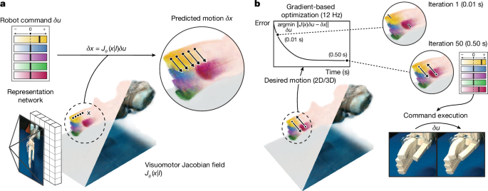
We define the dense 3D position of every robot point as the state of the robot. Consequently, the change in robot state δq can be interpreted as the 3D velocity field that moves these points under the action δu. The 3D velocity field δq can be measured as 2D pixel motions vⁱ across all camera views using off-the-shelf optical-flow and point-tracking methods. Given a training data sample (vⁱ, δu, Kⁱ, Pⁱ), our visuomotor Jacobian field J(x, I) associates the two signals (δq, δu) through \(\widehat\bfv^i=\rmrender\,(\,\bfJ(\bfX,\bfI),\delta \bfu,\bfK^i,\bfP^i)\) using equation 7, where X represents samples of 3D coordinates from the neural field.

To sum up, our Jacobian field leverages visual motion measurements as a learning signal and can be trained self-supervised purely by observing robot motion under random actions with multi-view cameras. It directly relates the change in robot state δq, defined as the 3D motion field that advects every 3D point of the robot according to the action δu, to the motion in 2D-pixel space observed by multiple cameras. This provides a signal for learning which part of 3D space is sensitive to a particular command of the robotic system, and enables control by specifying the desired motion of any robot point in 2D or 3D.

Trajectory tracking

Our MPC algorithm supports both 2D and 3D tracking tasks. The main differences lie in the choice of state representation and cost function. In both cases, the goal is to find the control input that best aligns the current observation with the next waypoint. Detailed procedures for demonstration preprocessing, state encoding and command optimization are provided in the Supplementary Information.

2D Trajectory tracking

For 2D tracking, we extracted point tracks from demonstration videos using TAPIR⁵⁸, guided by segmentation masks from a foundation model⁵⁹. At test time, TAPIR features were used to match or propagate points across frames. Jacobian fields predicted the motion for each pixel, and commands were optimized to minimize L2 distance to the target point locations. We accounted for visibility masks to ignore occluded keypoints.

3D Trajectory tracking

For 3D tracking, we lifted RGB video frames to 3D point clouds using PixelNeRF. Each waypoint was stored as a 3D point set sampled from high-density regions of the reconstructed volume. We optimized robot commands by minimizing the Wasserstein-1 distance^55,56 between the current and target point clouds. The Jacobian field was queried at each point to predict the advected cloud under a given control command.

Evaluations

Ablative baselines

Jacobian parameterization ablations

To understand why our Jacobian field enables better generalization and sample efficiency than direct scene flow prediction, we analysed the inductive biases embedded in its formulation. In particular, we studied how linearity⁴⁵, spatial locality⁶⁰ and compositionality^60,61—three key properties of mechanical systems—are naturally captured by our parameterization. We complemented these insights with experimental comparisons against a direct flow prediction baseline across real and simulated robotic systems^45,62. These results demonstrated that our approach generalizes substantially better than the alternatives to unseen robot configurations and commands. Full theoretical observations and experimental results are provided in the Supplementary Information.

Neural-rendering ablations

We ablated the neural-rendering part of the Jacobian fields by assuming that the model is given depth as input. Keeping the rest of the architecture unchanged, we trained a pixel-aligned 3D Jacobian fields model. This model was supervised using the same losses on depth and flow. We found that the baseline failed to disentangle the sensitivities of different surface points to different actuators, predicting incorrect Jacobians, probably because of a lack of multi-view supervision. Analysis and results are included in the Supplementary Information.

Analytical baselines

Allegro hand

We compared our learnt Jacobian field with an analytical Jacobian derived from the Allegro hand’s kinematic model using the Drake simulator⁴⁷. By aligning the predicted and analytical Jacobian fields through Procrustes analysis⁶³, we computed angular deviations between corresponding command-channel vectors. Our model achieved strong agreement, with an average error of 7° (Extended Data Fig. 6 and Extended Data Table 4). Details of the set-up and evaluation procedure are provided in the Supplementary Information.

HSA platform

We benchmarked our model against a 2D analytical-dynamics model of an HSA platform from previous work⁴⁸ that does not account for 3D twisting. We aligned the analytical and predicted Jacobian fields in 2D and evaluated vector alignment across sampled points. Our method robustly handled 3D motion and generalized beyond the limitations of the analytical baseline. Full methodology and results are provided in the Supplementary Information.

Robustness analysis

Robustness against visual occlusions

To improve the robustness to occlusion and background variation, we applied domain randomization techniques^64,65,66 during training by overlaying segmented robot foregrounds onto randomized backgrounds and natural scenes⁶⁷. Segmentation masks were obtained using the Segment Anything model⁵⁹. These augmentations improved the resilience of our neural 3D reconstruction module to visual clutter and partial occlusion. Empirical and quantitative results confirmed that depth and Jacobian predictions remained accurate despite such perturbations (Extended Data Fig. 3 and Supplementary Information).

Robustness against scene perturbations

We evaluated the ability of our system to generalize to substantial physical scene changes by testing control performance in a modified environment with altered geometry and appearance. Even with large occluders, such as cardboard fences, introduced at test time, our method accurately tracked 3D trajectories using the Allegro hand, achieving a median joint error of 2.89°. More information and experimental set-up are provided in the Supplementary Information.

Robot systems

We evaluated our method across four diverse robot platforms that had different actuation, morphology and modelling complexity. Full system details, including fabrication, control and sensing, are provided in the Supplementary Information.

Pneumatic hand

We used a pneumatically actuated soft robot hand that was 3D-printed in one piece by vision-controlled jetting⁶, based on the design in ref. ³⁰. It combined soft PneuNet fingers⁶⁸ with a rigid core and was controlled by 15 pneumatic channels. We used two configurations: a stationary hand and a version mounted on a UR5 robot arm.

Allegro hand

The Allegro Hand is an anthropomorphic robotic hand with 16 degrees of freedom that is widely used in research^69,70,71,72. It is commercially available and provides a challenging testbed, owing to its high degrees of freedom and mechanical dexterity.

HSA platform

This soft robotic platform with four degrees of freedom used handed shearing auxetic actuators³¹ that were 3D-printed by digital light projection⁷³. The platform’s compliant design enables wrist-like motions and linear extension, but accurate modelling is challenging owing to its deformation under external forces⁷⁴. It can be sensorized by fluidic innervation⁷⁵ or embedded cameras⁷⁶.

Poppy Ergo Jr

The Poppy Ergo Jr^32,77 is a low-cost, open-source robot arm with six degrees of freedom built using Dynamixel servos and 3D-printed parts⁷⁸. It is easily affordable but its mechanical tolerances and backlash make it difficult to model accurately^41,79,80.