A dependency map enhanced with next-generation 3D cancer models

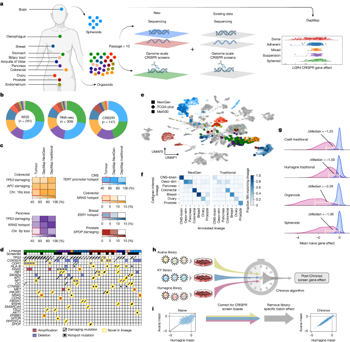
Source and culture conditions of NextGen cancer models

The source of each of the NextGen models is provided in Supplementary Table 1. In brief, breast cancer organoid models were derived by the laboratories of A.V.L., S.O. and D.L.S. Most of the NextGen CNS tumour models were derived by the laboratory of K.L.L. Colorectal and oesophagus–stomach cancer organoid models were derived by staff at the Cancer Cell Line Factory at the Broad Institute. Ovarian and uterus cancer organoid models were derived by the laboratory of S.J.H. Pancreas cancer organoid models were derived by the laboratories of A.J.A. and S.R. Prostate cancer organoid models were derived by the laboratory of H.B. and the laboratory of Y. Chen. Additional models derived by the HCMI were obtained via the American Type Culture Collection (ATCC). Models were confirmed for the absence of mycoplasma contamination (Mycoplasma PCR Detection kit; ABM, G238) and authenticated by short tandem repeat (STR) profiling (LabCorp) before expansion. These procedures were repeated monthly during expansion and screening.

Organoid media were prepared using the recommendations provided for each of the models (Supplementary Table 1). The conditioned media were prepared by culturing WNT3A-producing L cells (L Wnt-3A; ATCC, CRL-2647) and R-spondin-1-producing 293T cells (Cultrex R-spondin 1 (RSPO1) cells; Trevigen, 3710-001-K) in DMEM with 10% serum. After reaching 80% confluency, cells were washed once with PBS and incubated with Advanced DMEM–F12 medium (Thermo Fisher, 12634028) containing 100 mM HEPES, 1% penicillin–streptomycin and 1% 100× Glutamax (Ad+++) for another week. The conditioned medium from this culture was then collected, filtered and stored at –80 °C before being used for organoid cultures. All organoids were grown initially as domes composed of 75% growth-factor-reduced, Phenol Red-free Matrigel (50 μl per dome; Corning, 356231) in the recommended medium diluted 1:1 with Ad+++. The screening of organoids was conducted either in Matrigel dome cultures or in adherent cultures on Matrigel-coated plates (see the section ‘Genome-wide CRISPR screening of organoids’ below).

The NextGen CNS models were grown in tumour stem medium, the composition of which is described in Supplementary Table 1. The conditioned medium was collected routinely during expansion and preserved for subsequent cultures. Cells were seeded in a mixture of 30% conditioned medium and 70% fresh medium. Some of the models were tested for their ability to grow on a Matrigel-coated plate. In brief, cells were plated in 1% Matrigel-coated flasks and cells attached to the coating were carried forward as adherent models. Models that failed to attach to coated plates were grown as spheroids in ultra-low attachment (ULA) vessels (Corning, 3814). Models that were initially derived as adherent cultures on laminin-coated plates were maintained in the same conditions. To coat plates, Matrigel or laminin (Corning, 354232) was diluted in ice-cold PBS at a concentration of 1%. This solution was then added to culture vessels at approximately one-half the recommended volume of medium for a given vessel (for example, 5 ml solution in a T75 flask). Flasks were incubated at 37 °C overnight, and the solution was aspirated immediately before plating the cells. The growth format of each model is listed in Supplementary Table 1.

Preparation of samples for WGS and RNA-seq

To generate pellets from the organoids, the medium was first aspirated and then the Matrigel domes were scraped and transferred to a 20× volume of pre-warmed TrypLE (Thermo Fisher, 12604021) with 10 µM ROCK inhibitor (Peprotech, 129830-38-2). This mixture was incubated at 37 °C for 30 min. Subsequently, the cells were pelleted by centrifugation, resuspended in a mixture of medium and Matrigel and seeded at a density of 50,000 cells per dome. After 1 week of growth, cell pellets were collected without ROCK inhibitor for WGS and RNA-seq.

For the NextGen CNS tumour models, cells were seeded and propagated for 7–14 days, depending on their growth, and dissociated with TrypLE for 5 min at 37 °C. Following dissociation, the cells were counted, and the pellets of 1 × 10⁶ cells were collected and submitted for WGS and RNA-seq.

WGS analysis

WGS for all the DepMap NextGen models was conducted at the Broad Institute Genomics Platform using the PCR-free human WGS procedure. In brief, libraries were constructed and sequenced at 30× coverage on either an Illumina NovaSeq 6000 or NovaSeq X system, with the use of 150 base-pair paired-end reads. The FASTQ files from sequencing were de-multiplexed, aggregated and aligned using the DRAGEN germline pipeline to create BAM files.

Mutation calling from WGS

The mutation calls from the WGS results were generated using Mutect2 (ref. ⁶¹), annotated and filtered downstream. The detailed strategies are described in a publicly shared document (https://storage.googleapis.com/shared-portal-files/Tools/25Q3_Mutation_Pipeline_Documentation.pdf). In short, variants were aligned to the GRCh38.p14 human genome assembly (https://www.ncbi.nlm.nih.gov/datasets/genome/GCF_000001405.40/) and mutation calling was conducted with the following parameters: default format of VCF and HG38; Gatk_docker: broadinstitute/gatk:4.2.6.1; M2_extra_args:–genotype-germline-sites true–genotype-pon-sites true for getting access to germline calls; Filter_funcotations to False PoN: gs://gatk-best-practices/somatic-hg38/1000g_pon.hg38.vcf.gz; Run_funcotator to True; Run_orientation_bias_mixture_model_filter to True. The pipeline was run such that no bait sets were needed.

CN calling from WGS

Relative CN data were generated from the WGS data by running the GATK CN pipeline aligned to hg38 (ref. ⁶²). Absolute CN data from WGS or whole-exome sequencing were generated using PureCN⁶³. Arm-level CN values were calculated using PureCN segment-level CN as previously described⁶⁴. Gene-level amplifications were defined as having a relative CN (log₂[relative to ploidy + 1]) greater than 3, and deletions were defined as having a relative CN less than 0.25.

RNA-seq

RNA-seq for all the DepMap NextGen models was conducted at the Broad Institute Genomics Platform. In brief, poly-A RNAs were captured with oligo-dT beads, from which libraries (450–550 bp insert size) were prepared using a strand-specific Illumina TruSeq library preparation protocol. These libraries were sequenced to 100 million paired reads on either an Illumina NovaSeq 6000 or NovaSeq X system, with the use of 151 bp paired-end reads. The FASTQ files from sequencing were processed using the DRAGEN RNA-seq pipeline to create BAM files.

Source of traditional cell lines

The traditional cell lines used were obtained from DepMap, and the original source can be found on the DepMap portal (https://DepMap.org/portal). These included several commonly misidentified cell lines registered by the International Cell Line Authentication Committee (https://iclac.org/databases/cross-contaminations/). We reasoned that even though these cell lines are commonly misidentified, their inclusion in the DepMap dataset would be advantageous for comprehensiveness, provided they were confidently identified and authenticated. Accordingly, we performed STR profiling on the cell lines that are frequently misidentified. After confirming their identities, we decided to profile these lines and include their data in DepMap. Mycoplasma testing and STR profiling were performed after receiving the cell lines and every 3 months of culture period thereafter using a Mycoplasma PCR Detection kit (G238, ABM). Cells were grown in RPMI 1640 (Corning, 10-040-CV) supplemented with 2 mM glutamine, 50 U ml^–1 penicillin, 50 U ml^–1 streptomycin (Gibco, 10378016) and 10% FBS (MilliporeSigma, F4135) and incubated at 37 °C in 5% CO₂.

Lineage prediction with Celligner

To predict the lineage of cancer models (NextGen and traditional) using Celligner, the 25 nearest neighbour tumours from the TCGA, TARGET and Met500 datasets (n = 13,104) were identified for each model in Celligner’s aligned gene expression space according to pairwise Euclidean distance. For each lineage of the models, we computed the lineage representation among the neighbouring tumours as a global measure of model–tumour lineage similarity. To obtain per-model lineage predictions, we classified each model by the most frequent lineage found among its nearest neighbour tumours.

Models that fell into the ‘undifferentiated cluster’ were excluded in a part of the analysis shown in Extended Data Fig. 2a, as this cluster was highly enriched with adherent models from various lineages that exhibited loss of lineage-specific gene expression patterns, which made it difficult to predict lineages of the models in this cluster. The undifferentiated cluster was defined by applying the following criteria to the 79 clusters identified using Celligner: (1) number of DepMap models in the cluster > number of tumour samples in the cluster; and (2) average Hallmark epithelial mesenchymal transition ssGSEA enrichment score among the DepMap models in the cluster > 0.

This procedure identified four clusters with Celligner (clusters 28, 59, 62 and 67), which were collectively designated as the undifferentiated cluster.

Genome-wide CRISPR screening of organoids

After initial expansion and collection of viable stocks and pellets (used for fingerprinting and omics profiling; Extended Data Fig. 3), the organoids were tested for blasticidin sensitivity to identify the minimal concentration of blasticidin that gives less than 1% viability of uninfected cells in 10–14 days. Fourteen organoid models were screened as adherent cultures on Matrigel-coated plates, whereas the rest of the organoids were screened in 3D Matrigel dome cultures. To select the culture conditions for organoid screens, each of the organoid models was subjected to a growth format assay by seeding 50,000 cells into a well of a 24-well non-tissue-culture-treated plate (Corning, 351147) either as a Matrigel dome (75% Matrigel, 50 μl per dome) or on top of a Matrigel coat, referred to as either dome or coat format, respectively. The coated wells were prepared by first adding 1% Matrigel in ice-cold PBS to 50% of the standard filling volume of the well and allowing it to solidify by incubating overnight at 37 °C. Before cell plating, the PBS–Matrigel mixture was aspirated, leaving the Matrigel coat behind, and the cell suspension was added on top of the coat. The growth of cells in the dome and coat formats was compared after 1 week of culture via a viability assay with CellTiter-Glo 3D (3D CTG; Promega, G9683). Models with at least 30% viability on coat relative to dome format were propagated and screened in the coat format. This process enabled us to screen these models in a similar manner to traditional adherent cell lines, but with a thin layer of matrix support, thus decreasing the amount of required Matrigel by approximately tenfold.

Subsequently, all organoids were infected with lentivirus expressing enAsCas12a (Addgene, 136476). For this infection, 1.5 × 10⁶ cells were exposed to the lentivirus in a 24-well ULA plate (Corning, 3473) in the presence of 8 µg ml^–1 polybrene and 10 µM ROCK inhibitor. After 18 h, the cells were collected by centrifugation and washed once with PBS to remove the virus, and cells were then plated in Matrigel domes at 5 × 10⁴ cells per dome. At 24 h after seeding the cells in the Matrigel domes, the medium was replaced with selection medium containing blasticidin at 30 µg ml^–1. A 3D CTG assay was carried out 10–14 days after infection to ensure efficient elimination of uninfected cells with blasticidin and to measure the infection rate from the enAsCas12a virus. Cells were maintained at a constant blasticidin (as determined using a blasticidin sensitivity assay) concentration throughout the screening process.

Cas12a activity assessment was conducted as previously described⁶⁵ (a detailed protocol is available as ‘Cas9/Cas12a Activity Assay’ at the Broad Institute Genetic Perturbation Platform (GPP) web portal: https://portals.broadinstitute.org/gpp/public/resources/protocols) using two different types of lentivirus, both of which express GFP, a sgRNA (or sgRNAs) against GFP and the puromycin-resistance gene. One type of these virus expresses two GFP-targeting sgRNA sequences optimized for enAsCas12a (pRDA_221; Addgene, 169142), whereas the other virus type expresses a GFP-targeting sgRNA sequence optimized for spCas9 (pXPR-047; Addgene, 107145), the latter of which served as a negative control. Cells were infected with these two different virus types separately as described above and selected with puromycin for 4 days. GFP expression was measured in the FITC channel by flow cytometry (CytoFLEX LX, Beckman Coulter) 14 days after pRDA_221/pXPR_047 infection with a Zombie Aqua viability stain (BioLegend, 423102) applied to gate out dead cells. Using the non-infection control (NIC) as a negative control, GFP positivity was determined for both the pRDA_221 and pXPR_047 infected cells. Cas activity was calculated using the following formula: (GFP (%) of pXPR_047 – GFP (%) of pRDA_221)/(GFP (%) of pXPR_047).

Cell lines with Cas activity above 70% were selected for screening. However, some lines were screened with activity as low as 44% if they showed sufficiently rapid growth of at least one population doubling per week.

Library titrations were carried out to determine the volume of sgRNA library virus required to achieve an infection efficiency of around 50%. Infections were conducted on 24-well ULA plates, with each well containing 5 × 10⁵ cells in 600 µl medium with 4–8 µg ml^–1 polybrene, 10 µM ROCK inhibitor and 50–200 µl library virus. The plate was incubated at 37 °C for 18 h, followed by collection of the cells by centrifugation and a wash with PBS to remove the virus. Cells were subsequently plated in Matrigel domes on a 24-well plate. Puromycin (3 µg ml^–1) was added 48 h after virus infection. After 4 days of selection, infection efficiency was determined using a 3D CTG cell viability assay.

For the screens, cells were first infected using the same protocol as for library titration, but only with the virus volume selected to give an infection rate of about 50%. The number of cells used for infection was determined such that sufficient number of cells survived puromycin selection to produce at least 500× representation of the library. Before July 2022, the screens were performed using either the C or D versions of the Humagne library (Addgene, 172650 and 172651) at full representation for each library. By contrast, screens after July 2022 were performed in two technical replicates at half representation using a combined C and D library to enable measurement of replicate correlation. After 18 h of incubation with virus in ULA plates, the virus was washed out, and infected cells were plated at 5 × 10⁴ cells per dome. To test infection efficiency, we seeded four NIC domes and four infected domes in a 24-well plate (one dome per well). After 24 h, the medium was replaced with the selection medium containing puromycin for the infected plates and half of the domes (two NIC domes and two infected domes) for the infection efficiency assay. Puromycin was washed out and blasticidin treatment was resumed on day 6, when a 3D CTG viability measurement for the infection efficiency assay was conducted to estimate actual screen representation. Screens with less than 200× representation were excluded. The medium was replaced on days 13 and 20, and the samples were passaged on day 9 and optionally on day 17 depending on the confluence of the model, which was determined by visual inspection, each time maintaining minimum target representation. All the cells were collected and frozen as pellets on day 23.

gDNA samples were prepared from the screen pellets using a KingFisher Apex System (Thermo Fisher, 5400940). After preparing gDNA samples, the DNA concentration of each sample was measured using a Qubit4 Fluorometer (Thermo Fisher, Q33238), and the presence of library DNA was confirmed by performing PCR with a set of library-specific primers. gDNA samples were subsequently submitted for library DNA amplification and sequencing to the GPP at the Broad Institute. PCR and sequencing were performed in accordance with the ‘sgRNA/shRNA/ORF PCR for Illumina Sequencing’ protocol available at the Broad Institute GPP web portal (https://portals.broadinstitute.org/gpp/public/resources/protocols). DNA samples were sequenced at a scale matched with the size of the screen: 68 µg gDNA per replicate for screens with 500× representation and 134 µg gDNA per replicate for screens with 1,000× representation.

Genome-wide CRISPR screening of NextGen CNS tumours

The pipeline for genome-wide CRISPR screens of the NextGen CNS tumour models was adapted in part from previous work⁶⁶ and is composed of the same processes to what is described above in the section ‘Genome-wide CRISPR screening of organoids’ except for the following differences.

CNS models were tested for the growth format and seeding density that resulted in optimal growth rates and for polybrene sensitivity, which was used at a concentration that resulted in >85% survival. For growth testing, cells were plated in both Matrigel-coated and ULA 6-well tissue culture plates. Specifically, cells were seeded in duplicate at densities of 100,000, 200,000 and 300,000 cells per well for both the Matrigel-coated plates and ULA plates. Cells were allowed to grow for 7 days, with a medium change performed at day 3 or 4 as needed. After 7 days, cells from all the conditions were counted and a doubling time was calculated for each condition. The condition that gave the lowest doubling time while maintaining high cell viability was used for the screen. Blasticidin and puromycin were used at a standardized concentration of 50 µg ml^–1 and 3 µg ml^–1, respectively. For enAsCas12a transduction, 1.5 × 10⁶ cells were exposed to lentivirus expressing enAsCas12ain a 24-well ULA plate in the presence of the optimized concentration of polybrene. At 18 h after infection, cells were washed with PBS to remove the virus and the cells were plated in the optimal growth format at 2× the optimal seeding density. Subsequently, cells were selected with blasticidin. A CellTiter-Glo cell viability assay (CTG; Promega, G7572) was carried out 14 days after infection to ensure efficient elimination of uninfected cells with blasticidin and to measure the infection rate from the enAsCas12a virus.

For library titration, infections were conducted on 24-well ULA plates, with each well containing 1.5 × 10⁶ cells in 600 µl medium, the optimized concentration of polybrene and 50–200 µl library virus. The volume of virus required for an infection efficiency of about 50% was determined as described above in ‘Genome-wide CRISPR screening of organoids’. Blasticidin treatment was resumed on day 7 instead of day 6 after infection, and a CTG viability measurement for the infection efficiency assay was performed on the same day to estimate actual screen representation. Medium was replaced on days 10 and 17, and the samples were passaged on days 7 and 14, each time maintaining minimum target representation. All cells were collected and frozen as pellets on day 21, from which gDNA samples were prepared, and the library DNA was amplified by PCR and sequenced.

Genome-wide CRISPR screens of cancer cell lines

The original source for all the cell lines is available at the DepMap portal (https://DepMap.org/portal). The CRISPR screens of the traditional cancer cell lines with the spCas9 sgRNA libraries (Avana and KY) were carried out as previously described^67,68.

For the CRISPR screens of the traditional cancer cell lines with the enAsCas12a sgRNA library (Humagne-CD), the cell lines were first tested for doubling time and cell size. Blasticidin and puromycin were used at a standard concentration of 40 μg ml^–1 and 2 μg ml^–1, respectively. To infect adherent cells with lentivirus expressing enAsCas12a (Addgene, 136476), 5 × 10⁶ cells were exposed to the virus in a T175 flask (Corning, 354487) in the presence of 4 µg ml^–1 polybrene. For suspension cells, 1.8 × 10⁷ cells were exposed to the virus in a 12-well plate (Corning, 3513) in the presence of 4 µg ml^–1 polybrene, which was followed by centrifugation at 930g, 37 °C for 2 h. One day after infection, cells were washed with PBS to remove the virus and cells were then plated at around 50% confluence. Blasticidin was added to the medium 2–3 days after infection. A CTG assay was carried out after 3 days of blasticidin selection to ensure efficient elimination of uninfected cells with blasticidin and to estimate the infection rate from the enAsCas12a virus. Cells were maintained in blasticidin for at least 10 days after transduction and throughout the screening process. After enCas12a transduction and blasticidin selection, enCas12a activity was assessed as described in the section ‘Genome-wide CRISPR screening of organoids’.

Library titrations were performed in 12-well tissue-culture-treated plates, with each well containing 1.5 × 10⁶ cells in 2 ml medium, 4 μg ml^–1 polybrene and 0, 10, 25, 75, 200 or 500 μl virus. These 12-well plates were spun at 930g, 37 °C for 2 h, after which an additional 2 ml medium was added to each well for a final volume of 4 ml per well. After 24 h of infection, the cells in each well of the 12-well infection plate were split into 2 wells of a 6-well plate with 0 and 2 μg ml^–1 puromycin in fresh medium. An optimal seeding density was chosen such that the unselected population reached <70% confluence after selection. After 3 days of selection, infection efficiency for a given virus volume was determined as the ratio of live cells in the puromycin-containing well (2 μg ml^–1) to the number of live cells in the puromycin non-containing well. A linear regression of the virus volume to the transduction efficiency was performed to estimate the volume of virus required to transduce 50% of the population.

The remaining procedures of the screen were the same as for the procedures described above in the section ‘Genome-wide CRISPR screening of organoids’ except for the following modifications. For library infection, after 24 h of incubation with virus in 12-well plates, the virus was washed out with PBS and infected cells were plated with puromycin at an appropriate seeding density and flask size. After 72 h of selection, puromycin was washed out and blasticidin treatment was resumed. Screens with less than 250× representation or at an infection efficiency of higher than 60% were excluded. Cells were passaged every 3–6 days depending on the confluence of the model, as determined by visual inspection, each time maintaining minimum target representation. All cells were collected and frozen as pellets on day 22–23.

Genome-wide CRISPR screening data processing and quality control evaluation

All screens were initially evaluated for sequencing quality and selected to have a mean of at least 185 reads per gene. Naive gene effect scores were calculated by taking the log of the ratio of normalized reads for each gene in screened samples to that of normalized reads for each gene in the corresponding plasmid library. For screens using the two Humagne C and D libraries, the log fold change scores of libraries were averaged together. An ROC-AUC was calculated on the basis of per cent of true positive hits (essential genes with log fold change below –1) for every possible false discovery rate. An NNMD was calculated for each screen by taking the difference between the average log fold changes for essential and non-essential genes and dividing by the standard deviation of the non-essential genes⁶⁹. Screens that had an NNMD greater than –1.25 or a correlation between replicates less than 0.19 were excluded from downstream analyses. Chronos scores were then calculated using the open-source code Chronos (v.2.0.8; https://github.com/broadinstitute/chronos) as previously described²³ for each type of guide library (Avana spCas9, KY spCas9 or Humagne CD enAsCas12a) independently. To mitigate batch effects between guide libraries, the mean Chronos score per gene in individual libraries was regularized towards the global mean across all libraries. On the DepMap portal, the file ‘ScreenGeneEffect’ contains Chronos gene effect estimates for each individual screen, with library effects corrected out whereas organoid-specific effects are preserved. Beginning with the 26Q1 release, a similar strategy will be used to preserve organoid-specific effects in ‘CRISPRGeneEffect’, which integrates all screens of the same model into a model-indexed table that can be used with portal tools.

Comparison of gene expression profiles between spheroid and adherent cultures of the NextGen CNS models

Nine NextGen CNS models were adapted to grow as adherent cultures on Matrigel-coated plates (coat culture) for 4 weeks or more. RNA samples were collected both before and after adaptation and profiled by RNA-seq using a similar protocol as described above. For these 18 samples (nine models × two conditions (spheroid and coat)), a correlation matrix was calculated based on the expression of the top 10% highly variable genes (n = 1,919). Subsequently, hierarchical clustering of the correlation matrix was conducted using the hclust and heatmap.2 functions in R (Extended Data Fig. 4c). To compare the expression levels of individual genes between the nine samples of spheroid culture and the nine samples of coat culture, the difference in expression levels of all the genes measured in this analysis (n = 19,193) were analysed using two-tailed Mann–Whitney U-tests (Extended Data Fig. 4f).

Comparison of gene dependency profiles between different growth formats of NextGen CNS models and organoids

For the NextGen CNS tumour models and organoids, the gene dependency profiles were compared between the two different culture conditions used for each of these model groups. Specifically, for the NextGen CNS models, the dependency scores between spheroid culture (n = 14) and coat culture (n = 25) and for organoids, and the dependency scores between Matrigel dome culture (n = 55) and coat culture (n = 14) were compared for every gene assessed in the CRISPR screen of these models (n = 18,159) using two-tailed Mann–Whitney U-tests (Extended Data Fig. 4h). For the organoids in Matrigel dome cultures, only the models from lineages that have corresponding coat-cultured models (ampulla of Vater, colorectal, oesophagus–stomach, ovary, prostate and uterus) were included in this comparison.

Classification of dependency profiles

The classification of dependency profiles (Extended Data Fig. 5a) was conducted primarily based on a published strategy²⁵ using the entire set of the NextGen (n = 147) and organoid (n = 108) models. First, we identified a negative control set of non-expressed genes per model as having a log₂[TPM + 1] expression value of less than 0.2. We then inferred the probability that the score represents a true dependency by using an expectation–maximization step until convergence independently in each screen or model. The dependent distribution was derived from the list of essential genes, which was generated from the intersection of previously published lists of essential genes^70,71. The null distribution was determined from non-expressed gene scores for the respective model if the expression data were available, or otherwise from the non-essential gene list inferred from a published study⁷⁰.

To identify pan-dependencies, we selected a gene rank threshold T based on the dependency rank of all the genes in their 90th percentile least depleted model. The distribution of this 90th percentile rank was bimodal, and T was defined as the rank that gives the minimum density between the two peaks. To identify high variance genes, we first selected an expression threshold by analysing the distribution of expression values across all NextGen (or organoid) models, which was bimodal, and selecting the value corresponding to the minimum density between the two modes. Genes with average expression less than this value were designated as lowly expressed. The variance threshold V was determined as the 99th percentile variance over lowly expressed genes. To identify strongly selective genes, we computed the product S of the skew and kurtosis of the distribution of gene dependencies over all NextGen (or organoid) models for each gene.

Using the scores defined above, we classified the genes in the following order:

1. 1)

   Pan-dependency: ranked in the 90th percentile least depleting line above T.

2. 2)

   Strongly selective dependency: S < –0.86, has a probability of dependency >0.5 in at least three models, and does not meet criterion (1).

3. 3)

   High variance dependency: the variance in the dependency score is above V and does not meet criteria (1) or (2).

4. 4)

   Weakly selective dependency: has a probability of dependency >0.5 in at least one model and does not meet criteria (1)–(3).

5. 5)

   Non-dependency: probability of dependency <0.5 for all models and does not meet criteria (1)–(4).

Identification of biomarker-associated dependencies

To identify dependencies with expression addiction, we scored the Pearson’s correlation coefficient (r) and the significance (P) of correlation between the expression level (log₂[TPM + 1]) and dependency (Chronos gene effect) of the same gene across all the NextGen models that were profiled by both RNA-seq and CRISPR screening (n = 146) (Fig. 2a). This process was conducted for all the genes that have expression data and were classified as strong dependency (strongly selective, high variance or pan-dependency) in the NextGen model CRISPR screen dataset (n = 3,786). The false discovery rate (or q value) was calculated using the Benjamin–Hochberg procedure for this and subsequent analyses unless otherwise indicated. The genes that met the criteria for significance (r < −0.3 and q < 0.005) were identified as dependencies with expression addiction. For each of the strong dependency genes identified from the NextGen model data, the correlation between expression and dependencies was also computed across the profiling results of the traditional cell lines that have lineage-matched NextGen models and gene expression data (n = 572).

Paralogue dependencies were identified by calculating the Pearson’s correlation coefficient and the significance of correlation between the dependency (Chronos gene effect) on a gene and the expression level (log₂[TPM + 1]) of its paralogue partner (Fig. 2d). We conducted this process for all the strong dependency genes in the NextGen model CRISPR screen dataset (n = 3,800), comparing their dependency with the expression level of the respective paralogue partners listed on Ensembl genome browser 113 (https://www.ensembl.org/). Paralogue pairs were extracted via BioMart query for all human paralogues with valid HGNC symbols. Only gene pairs with at least 25% sequence identity between paralogues and with variance in expression >1 over all the NextGen models were considered for analyses. The dependency gene–paralogue pairs that met the significance criteria (r < –0.3 and q < 0.005) were identified as paralogue dependencies. Here again, we computed correlations for the same dependency–expression paralogue pairs in the traditional model profiling results (n = 572).

To find dependencies that are associated with oncogene GOF or TSG LOF, we first identified models with oncogene GOF as either harbouring a hotspot mutation or CN gain (log₂[relative to ploidy + 1] > 3) of the oncogene, and TSG LOF as either having a damaging mutation or CN loss (log₂[relative to ploidy + 1] < 0.25) of the TSG for all the oncogenes and TSGs listed in OncoKB¹ (https://www.oncokb.org/). We selected 6 oncogenes and 13 TSGs that had at least 1 model of hotspot mutation and 5 or more models of relevant alteration among the NextGen models with CRISPR screen profiles (n = 147). For each of these oncogenes and TSGs, we assessed whether any of the strong dependencies were significantly enriched in the NextGen models with the respective cancer gene alteration (‘altered’) compared with the rest of these models (‘unaltered’) using two-tailed Mann–Whitney U-tests with a threshold of q < 0.05 (Fig. 2f).

To test whether the observed association between the cancer gene alteration and dependency was consistently beyond the effects caused by lineage bias of the cancer gene alteration, we also computed the differences in mean dependency between NextGen screens in each lineage and the remaining NextGen screens, only considering lineages that have at least five models screened. If the dependency difference observed across the two classes of models distinguished by the presence of a cancer gene alteration was outside the range of all dependency differences observed across all lineages, then we deemed the dependency–biomarker relationship to be driven by the cancer gene alteration. Otherwise, the dependency pattern was attributed to lineage effects. The mean dependency scores for the altered and unaltered groups, as well as the significance of these mean dependency scores, were similarly calculated for all these 6 oncogenes and 13 TSGs in the traditional models (n = 597).

SCD inhibitor sensitivity assay in oesophageal adenocarcinoma organoids

To examine whether the increased reliance on SCD of oesophageal adenocarcinoma organoids with KRAS CN amplification, identified via CRISPR screens, can be reproduced with pharmacological SCD inhibition, we tested two chemical inhibitors of SCD: A939572 and CAY-10566. Specifically, we tested four oesophageal adenocarcinoma models, two with KRAS CN amplification (CCLFUPGI0012T and CCLFUPGI0030T) and two with neutral KRAS CN (CCLFUPGI0022T and HCMSANG0300C15). On day 0, for each of these four models, 10,000 cells per well were seeded into 120 wells of 96-well ULA plates (Revvity, 6055802) in a slurry culture with 100 μl of 5% Matrigel–OPAC per well. One of the following compounds was added to the culture at the same time as seeding using a D500e Digital Dispenser (Tecan Life Sciences): A939572, CAY-10566 and bortezomib. For each of these compounds, nine different doses with serial dilutions (2 nM to 10 μM, 2.9-fold dilution between the neighbouring doses) and DMSO control were tested in quadruplicate. On day 3, 50 μl fresh medium containing the corresponding concentration of the compounds was added to the culture.

To measure viability of cells following compound treatment, 50 μl 3D CTG assay reagent was added to the culture and mixed by pipetting on day 7. This was followed by an incubation of the plates at room temperature (RT) for 30 min on a digital microplate shaker (Thermo Scientific, 88882006) at 300 rpm. Subsequently, luminescence emission was measured using a CLARIOstar Plus plate reader (BMG LABTECH).

Scoring the activity of gene expression MPs

We used a published method³⁷ to score the activity of 41 different gene expression MPs in each of the tumour samples and culture models. In brief, MP scores were calculated as the average relative expression of the MP gene set minus the average relative expression of a control gene set; that is,

in which MP_i,j indicates the score of MP_j in sample i, G_j is the gene set for MP_j and Ctrl_j is a control gene set for MP_j. To define the control gene set, all analysed genes were grouped into 25 bins on the basis of their mean expression levels. Subsequently, for every gene in the MP gene set, 100 genes were selected randomly from the same expression bin to constitute the control gene set.

MP expression across different sample types (for example., traditional versus NextGen models, 2D models versus organoids, tumours versus traditional models, tumours versus NextGen models, GBM tumours versus GBM models with specific gene expression subtype, and between different subtypes of oesophagus–stomach tumours) (Figs. 3a and 4a,b and Extended Data Figs. 6d and 7d,e) were compared using two-tailed Mann–Whitney U-tests.

NextGen GBM model dependency analyses

To analyse gene expression and associated dependencies in the NextGen GBM models, the transcriptional landscape of GBM models was visualized in a 2D UMAP using Celligner embedding (Fig. 3b). The cohort included 55 traditional and 70 NextGen GBM models, alongside 189 tumour samples from the TCGA-plus and Met500 GBM cohort. Two clusters were identified visually on the UMAP plot on the basis of distinct groupings of data points. Differential gene expression analysis was conducted to compare the transcriptional profiles of the clusters by computing log₂ fold changes to quantify expression differences and performing two-tailed Student’s t-tests to assess significance for each gene. Significance was determined using adjusted P values (q values), with thresholds applied at q < 0.001 and |log₂[fold change]| > 1 (Fig. 3c).

Differential dependency analysis was performed between the glial GBM models (screen n = 36) and either mesenchymal GBM models (screen n = 60) (Fig. 3d) or all the other non-glial NextGen models (organoids and non-glial NextGen CNS models; n = 115) (Extended Data Fig. 6e). Common essential genes were excluded from the analysis. Significant dependencies (effect size < –0.3, q < 0.05; P < 0.05 cutoff was also used for Fig. 3d) were identified and visualized using a volcano plot.

To identify a CN of a gene that can serve as a biomarker to predict CDK6 dependency, the Pearson’s correlation between CDK6 dependency and CN of genes (only those in the top 10% high variance of CN in the DepMap GBM models) was calculated and plotted across DepMap GBM models (with CRISPR and CN data; n = 95; Fig. 3f). The correlation between CDK6 dependency and CN of genes was similarly calculated using only the DepMap GBM models that exhibited the glial pattern of gene expression (n = 36; Extended Data Fig. 6g). Associations with |r | > 0.3 and q < 0.05 were considered as significant. We also analysed the difference in CDK6 dependency between mutant and non-mutant screens for all the hotspot or damaging mutations that have ≥5 mutant cases in the DepMap GBM models (5 mutations met this criterion; Extended Data Fig. 6f) again using the data from the entire DepMap GBM model cohort. None of these mutations was significantly associated with CDK6 dependency (all q > 0.95 by a two-tailed Mann–Whitney U-test).

CDK6 dependency validation in patient-derived short-term cultures

We used seven patient-derived (NextGen) GBM models (BT286, BT179, BT145, BT320, BT444, BT224 and BT187) to evaluate their sensitivity to CDK4/6 inhibition. Patient-derived models were maintained at 37 °C and 5% CO₂. Cells were plated at 500–2,000 cells per well in 60 µl medium in 384-well CellCarrier plates (Perkin Elmer, 6057302) and allowed to adhere for a minimum of 24 h. Cells were then treated with drugs in half-log dilution series with a D300 digital drug dispenser (Hewlett Packard). Palbociclib, ribociclib and abemaciclib (MedChem Express, HY-50767, HY-15777, HY-16297A, respectively) were identity and purity verified by LC–MS and prepared as 10 mM stocks in DMSO. Palbociclib was diluted to 5 mM before dispensing owing to solubility limitations. At the time of drug addition, a time = 0 control plate was fixed. Following 96 h or 120 h in drug, treated plates were fixed.

Plates (both time = 0 and treated plates) were stained, fixed, imaged and analysed according to the Dye Drop or Deep Dye Drop protocols⁴³. In brief, for Dye Drop, cells were stained with Hoechst 33342 (1:5,000, Thermo Fisher, 62249) and LIVE/DEAD far red fluorescent dye (LDR, 1:2,000, Thermo Fisher, L10120), prepared in a 10% solution of OptiPrep (Sigma, D1556) in PBS to displace the growth medium, for 30 min at RT. Cells were then fixed with 4% formaldehyde, prepared in 20% OptiPrep (a denser solution to displace the stain solution and media column), for 30 min at RT. Fix, stain and medium were aspirated and 80 µl PBS was added per well. Plates were then sealed and stored at 4 °C until image acquisition. For Deep Dye Drop, cells were stained with LDR and pulsed with EdU (Lumiprobe, 30540) in a 10% solution of OptiPrep in PBS for 1 h before fixation with 4% formaldehyde, prepared in 20% OptiPrep for 30 min. Wells were aspirated and cells were then permeabilized with 0.5% Triton X-100 (Sigma, T8787) in 10% OptiPrep for 20 min at RT, and EdU was then labelled with cy3-azide (Lumiprobe, C1030) by Click chemistry in 20% OptiPrep for 30 min at RT. Following aspiration, cells were blocked in Odyssey buffer (LI-COR Biosciences, 927-40150) for 1 h at RT, and then stained with anti-phospho histone H3 Alexa 488 (pH3, 1:2,000, Cell Signaling Technologies, 3465S) and Hoechst 33342 (1:5,000) overnight at 4 °C. Cells were washed once with PBST, twice with PBS and sealed for storage at 4 °C until image acquisition. All wash steps were performed with an EL406 washer equipped with a 96-channel head (Biotek).

Images were acquired on an Operetta (Perkin Elmer) with a ×10 objective. Six fields of view were imaged per well. Nuclear segmentation was performed based on Hoechst intensity with Columbus (v.2.7.0, Perkin Elmer). A ring around the nucleus was drawn and the intensity of each marker was measured in the nuclear and ring masks. The intensity in the ring was subtracted from the nuclear intensity to correct for deviations in local background intensities. Cells were classified as live or dead on the basis of LDR signals, cells positive for EdU or pH3 were classified as S phase or M phase, respectively, and the integrated Hoechst intensity was used to measure DNA content and to assign cells doubly negative for EdU and pH3 to the G1 (DNA content = 2N) or G2 (DNA content = 4N) phases of the cell cycle. Cells negative for EdU with intermediate DNA content were assigned ‘S dropout’. All gating was performed with custom Python scripts that are publicly available (https://github.com/datarail/DrugResponse/wiki). Live cell counts were used to calculate growth rate inhibition values⁷².

PDAC-classical/MUC program expression analyses

To assess the relationship between PDAC-classical/MUC program expression and the classical score (based on a previously defined ‘classical’ gene set⁴⁶) of tumour samples, the classical score was determined using the same strategy as the calculation of the MP expression score described above (in the section ‘Scoring the activity of gene expression MPs’). The relationship between the purity of tumour samples and the level of PDAC-classical/MUC program expression was analysed by compiling the ABSOLUTE tumour purity score of the TCGA tumour samples of pancreas, oesophagus–stomach and colorectal lineages (n = 149, 375 and 448, respectively) from previous studies^59,73.

The expression levels of the PDAC-classical/MUC program in various sample types (tumours, NextGen models and traditional cell lines) were also visualized by the colour of the points on the Celligner plots (Fig. 4c and Extended Data Fig. 7c) to show the similarity of the overall gene expression profiles of the models and tumours displaying high expression levels of this program across different lineages (pancreas, oesophagus–stomach and colorectal).

Dependencies associated with PDAC-classical/MUC program expression

To identify genetic dependencies associated with the level of PDAC-classical/MUC program expression, the Pearson’s correlation coefficient and the significance of correlation (two-tailed) were calculated between the level of the PDAC-classical/MUC program and the dependency scores of strong dependency genes (strongly selective + high variance + pan-dependency; n = 3,521) identified from the organoid screen data using all the organoid models with gene expression and CRISPR screen data (n = 108 (all organoids), n = 60 (organoids grown with R-spondin 1 and WNT3A); Fig. 4d and Extended Data Fig. 7i). The enrichment of the MSigDB gene set ‘GOBP WNT signalling pathway’ in the dependencies associated with PDAC-classical/MUC program expression was assessed by gene set enrichment analysis, which was conducted using the open-source code GSEApy (v.1.1.5; https://pypi.org/project/gseapy/) (Fig. 4d).

The PDAC-classical/MUC program-associated dependencies on the selective components of the WNT signalling pathway, namely TCF7L2, WLS, FZD5 and MESD (plus LGR4 for some analyses), were investigated further as follows. The dependency on these WNT pathway components were compared between the organoid models (n = 108) and the traditional cell lines that have lineage-matched organoid models (screen n = 485) using the density plots and two-tailed Mann–Whitney U-tests (Fig. 4f). To test whether dependencies on these WNT pathway components observed in organoids (with high levels of PDAC-classical/MUC program expression) is driven by specific mutations, 14 hotspot mutations and 573 damaging mutations that have 2 or more mutant models in the cohort of CRISPR-screened organoids (n = 108) were selected. For each of these 587 mutation types, dependencies on the 5 WNT pathway components listed above were compared between the mutant and non-mutant models (Extended Data Fig. 7k). For mutations and CN alterations that result in the activation of the WNT pathway, namely, APC damaging mutation, CTNNB1 hotspot mutation, CTNNB1 CN amplification and RNF43 damaging mutation, dependencies on TCF7L2, WLS, FZD5 and MESD were also compared between the organoids that have at least one of these alterations (n = 30) and those that do not have any of them (n = 78) (Extended Data Fig. 8a,b).

Cancer gene dependencies in 3D organoids versus 2D models

To compare dependencies on cancer genes (that is, oncogenes and TSGs) between the 2D models (screen results from traditional adherent models that have lineage-matched 3D organoids; n = 433) and organoids (n = 94), 90 cancer genes (40 oncogenes and 50 TSGs) with frequent (>1%) mutation rates in the TCGA cohort were selected based on a previous publication⁵³. CDKN2B was not included as none of the organoids has a CRISPR screen result for this TSG. The dependencies on each of these cancer genes were compared between the 2D models and 3D organoids. The significance of the difference was assessed using two-tailed Mann–Whitney U-tests. For the cancer genes for which mutation (hotspot mutation for the oncogenes and damaging mutation for the TSGs) is annotated in DepMap, the same analysis was conducted after removing the mutant models to see whether the differing dependencies between the 2D models and 3D organoids is attributable to the differing rates of mutation between these two model types (Extended Data Fig. 8d).

To assess whether 2D models and 3D organoids exhibit difference in dependencies on a group of oncogenes or TSGs in the same signalling pathway, each of the 89 cancer genes frequently mutated in TCGA tumours were classified into one of the ten oncogenic signalling pathways based on the function of the protein they encode⁵³. For the groups of oncogenes and the groups of TSGs that belong to the same pathway (13 groups), mean dependency scores for the genes in the same group were calculated for each model. Subsequently, the mean dependency scores of the 2D models and 3D organoids were compared using two-tailed Mann–Whitney U-tests (Extended Data Fig. 8f).

Differential dependency analysis between 3D organoids and 2D models

To identify functional classes that are enriched for genes exhibiting differing degrees of dependency between 2D models (screen results from traditional adherent models that are lineage-matched with 3D organoids; n = 433) and 3D organoids (n = 94), we ranked all genes (n = 16,691; excluding common essential genes) according to their mean difference in dependency score between organoid models and lineage-matched adherent models. The genes with the 100 most extreme differences in each direction were combined into one set. Gene sets from the Hallmark and KEGG legacy collections, which contain 101–249 member genes that were ranked in this analysis, were tested for enrichment among this set of 200 genes using a hypergeometric test (or one-sided Fisher’s exact test). The gene sets that achieved significance at q < 0.05 were compared for similarity using the overlap coefficient:

Gene sets with pairwise overlap similarity >0.3 were identified as belonging to the same functional cluster (Extended Data Fig. 8h). Clusters were successively combined using their original component gene sets until all clusters contain no gene sets having similarity >0.3 with any gene sets belonging to a different cluster.

Lentiviral production for the minipool screen and its validation

Lentiviral production was conducted using 293FT cells (Thermo Fisher, R70007) in accordance with the ‘Lentiviral Production in Flasks’ protocol available at the Broad Institute GPP web portal (https://portals.broadinstitute.org/gpp/public/resources/protocols). In brief, the lentiviral particles were generated by the co-transfecting the lentiviral plasmid with a packaging plasmid (psPAX2; 12260, Addgene) and VSV-G envelope (pMD2.G; Addgene, 12259) into 293FT cells using PEIpro transfection reagent (Polyplus, 101000033). The medium was replaced 12 h after transfection, and the virus-containing medium was collected after 36–48 h.

Library preparation for minipool screens

For the minipool screens, to evaluate the effects of growth formats and culture media on gene essentiality, we decided to select test genes from nine different functional classes. Most of these gene classes are related to the regulation of adhesion–cytoskeleton, lipid metabolism or other processes highlighted in the systematic comparison of genome-wide CRISPR screen data between 2D models and 3D organoids (Fig. 5a,b). The following gene classes were included: integrin (genes encoding an integrin α or β subunit); ECM adhesion (adhesome, https://adhesome.org/); actin regulation (MSigDB gene set and KEGG regulation of actin cytoskeleton); adherens junction (MSigDB gene set and KEGG adherens junction); tight junction (MSigDB gene set and KEGG tight junction); lipid metabolism (a union of two MSigDB gene sets, Hallmark cholesterol homeostasis and Reactome metabolism of lipids); WNT signalling (MSigDB gene set and GOBP WNT signalling pathway); PI3K–mTOR signalling (MSigDB gene set and Hallmark PI3K–mTOR signalling); cell cycle (MSigDB gene set and GOBP cell cycle); and other genes of particular interest (manual curation). To select 250 test genes from these 9 core functional gene classes, we used the dependency profiles of the gene between 2D models and 3D organoids to prioritize genes that exhibited selective enrichment of dependency in either of these model types. Many of these test genes belong to multiple different classes, and the patterns of membership of individual genes across the nine classes and the number of test genes that exhibit the specific pattern are presented in Extended Data Fig. 9a. We then added 650 non-dependency genes and 100 pan-dependency genes, genes that are universally essential across 2D models and 3D organoids, to compile a list of 1,000 genes (Supplementary Table 3). We subsequently designed 4 enAsCas12a sgRNA sequences for each of these 1,000 genes using the CRISPick web tool (https://portals.broadinstitute.org/gppx/crispick/public), which were assembled into 2 constructs (2 sgRNA sequences for the same gene per construct; 2 constructs per gene) of the pRDA_052 backbone (Addgene, 136474). The resulting library with 2,000 constructs was used for minipool screening.

Minipool screening

Before screening, models were tested for their growth in an alternative medium (1:1 OPAC organoid medium for 2D models and RPMI with 10% FBS for 3D organoids) and with alternative growth format (3D Matrigel dome growth for 2D models and 2D monolayer growth for 3D organoids) for at least two passages. Only the combination of medium type and growth format that enabled a comparable rate of growth with the original conditions (<2-fold difference in the doubling times) and reasonably rapid growth (doubling time <120 h), as well as the original conditions of growth format–culture medium pair, were used for the screening. Moreover, all the models selected for screening were subjected to titrations of library virus and puromycin to determine the dose of virus to achieve optimal infection rates and the concentration of puromycin to kill uninfected cells within 3 days, respectively.

For the screen, selected models were infected with the amount of library virus required for infecting 30% of the cells in accordance with the result of virus titration on day 0. The infected cells were selected with the concentration of puromycin determined in the puromycin titration between day 1 and day 4. On day 4, cells were seeded into up to 4 conditions (2D monolayer culture on plastic plates (plastic culture) with RPMI + 10% FBS (RPMI–FBS); plastic culture with 1:1 OPAC; 3D Matrigel dome culture (dome culture) with RPMI + 10% FBS; and dome culture with 1:1 OPAC), depending on how many conditions survived the above-mentioned selection criteria for the respective model. For plastic culture, 2 million cells were resuspended with 10 ml of the respective medium and seeded on a Falcon 100 mm TC-treated cell culture dish (Corning, 53003). For dome culture, 2 million cells were resuspended with 0.5 m of the medium used for the condition and subsequently mixed with 1.5 ml of Matrigel. Approximately 40 domes, each with 50 µl of Matrigel–cell suspension were placed on a 100 mm TC-treated culture dish, which was followed by the incubation of the plate at 37 °C for 30 min to allow the Matrigel to solidify. Subsequently, 10 ml of the culture medium was added before further incubation. We prepared two technical replicates per each condition.

These cultures were maintained until day 14 with refreshment of the medium every 3 days. If the culture showed signs of confluency (coverage of more than 80% of the bottom surface by the cells for monolayer culture on plastic plates and appearance of a dark spot in the middle of the domes for Matrigel dome culture), we passaged the cells instead of replacing the medium while keeping the number of cells after passaging to 2 million cells per dish. Trypsinization (with 0.25% trypsin and 0.1% EDTA (Corning, 25-053-CI)) was used for the passaging of cells in plastic cultures, whereas cells in dome cultures were passaged in accordance with the strategy described above in the section ‘Source and culture conditions of NextGen cancer models’. At day 14, cells were collected by trypsinization and counted. gDNA samples were prepared from these cells and the abundance of individual sgRNA sequences in the genome of these cells were analysed by PCR amplification of the sgRNA sequences, preparation of sequencing libraries from the PCR products and subsequent sequencing of these libraries as described in the section ‘Genome-wide CRISPR screening for gDNA isolation and sequencing’.

Minipool screen analysis

Minipool screens were evaluated for sequencing quality by having a total read count of at least 500,000 reads across replicates. Gene scores and NNMDs were computed in the same manner as the genome-wide screens. Replicate correlation was computed as the Pearson’s correlation coefficient over log fold changes in all non-control genes. Screens with NNMDs greater than –1.5 and replicate correlations less than 0.2 were excluded from downstream analyses. Screens with a single replicate were retained if their other metrics passed these quality control thresholds. Chronos scores were calculated as previously described²³, with adjusted hyperparameters (smoothing regularization parameter = 0.3, kernel width = 5) for the smaller library size. Subsequently, we modelled the Chronos score Y_g,k for each gene g and screen k with the generalized linear regression model:

The first term captures the baseline viability effect of knocking out gene g. The second and third terms capture the growth format effect and medium effect, where I_d and I_s are indicator variables representing the types of growth format (Matrigel dome culture (dome) versus monolayer culture on plastic plates (plastic)) and culture medium (serum-free OPAC medium versus serum-containing RPMI–FBS medium), respectively. The fourth term captures interaction effects between these two conditions, and the final term captures model effects to account for multiple screens in the same cell line. Differences in effect sizes across growth format and serum status were extracted as β_d and β_s, respectively. Significance values corresponding to the same coefficients were extracted from the P values calculated using two-sided linear regression t-test.

To assess the effects of growth format (or culture medium) on the core functional classes of gene targets included in our minipool library, we calculated the variance in β_d (or β_s) across members of the same class and compared it to the variance in β_d (or β_s) across all non-control genes outside of class. For each gene set, we tested whether the in-class variance was significantly greater than the out-of-class variance using one-tailed F-tests.

Single-gene validation viability assay

The viability effect (10 days after sgRNA transduction) of CRISPR-mediated knockout of ITGB1, ITGAV, MSMO1 and SQLE (Fig. 5h and Extended Data Fig. 10a) was assessed using CTG cell viability assays. Specifically, KP3 and HS766T pancreatic cancer cells, both of which were engineered to express enAsCas12a, were infected with several different types of sgRNA-expressing lentivirus on day 0, which included CRISPR cutting controls (sgCh2 and sgAAVS1), sgRNAs targeting common essential genes (sgPOLR2D, sgSF3B1 and sgKIF11) and sgRNAs against the experimental genes (sgITGB1, sgITGAV, sgMSMO1 and sgSQLE). The infected cells were selected with 2 μg ml^–1 puromycin between day 1 and day 3. On day 3, cells were trypsinized, counted and reseeded without puromycin. For the 2D monolayer culture on a plastic plate (or plastic culture), cells were seeded at 2,000 cells per well in 100 µl RPMI medium with 10% FBS onto an opaque 96-well plate (Corning, 3903). For the 3D Matrigel dome culture (or dome culture), 10,000 cells were resuspended with 50 μl Matrigel and plated as a dome onto a 12-well plate, which was subsequently incubated (Corning, 356231) at 37 °C for 30 min to allow the Matrigel to solidify. The Matrigel dome was then covered with 1,200 μl per well of either the RPMI medium with 10% FBS or the 1:1 OPAC medium before further incubation. The medium was replaced every 3 days until day 10. Puromycin (2 μg ml^–1) was added back to the culture at the first medium replacement.

On day 10, the medium of the plastic-cultured cells was replaced with 100 μl per well of fresh RPMI with 10% FBS, and 40 μl per well of CTG assay reagent was subsequently added. Following incubation at RT for 30 min with constant shaking, luminescence emission was measured using a SpectraMax M5 Multi-Mode microplate reader (Molecular Devices, M5). For the dome-cultured cells, the medium was replaced with 350 μl per well of fresh RPMI with 10% FBS and 350 μl per well of 3D CTG assay reagent was subsequently added. Following incubation at RT for 30 min with constant shaking, the dissolution of Matrigel was confirmed by microscopy. Next, 150 μl of the lysate was transferred to an opaque 96-well plate to measure luminescence emission via a microplate reader. The luminescence signal from each of the experimental wells was normalized using a scale in which the average value of the cutting control wells (six wells; triplicate wells for each of sgCh2 and sgAAVS1) was scored as 0 and the average value for the common essential control wells (nine wells; triplicate wells for each of sgPOLR2D, sgSF3B1 and sgKIF11) was scored as −1. The normalized viability score for each of the experimental wells was plotted. The relative viability scores before normalization were also plotted (Extended Data Fig. 10a). The experiments were repeated twice. Each of these experiments was conducted with technical replicates (n = 3).

Immunofluorescence and flow cytometry of single-gene validation

For immunostaining of cells grown in either plastic culture or the dome culture conditions, cells were propagated on a Nunc 8-Well Lab-Tek chamber slide (Thermo Fisher, 177402). For plastic culture, the slide was first incubated with 100 μg ml^–1 collagen I (Corning, 354236) and 20 μg ml⁻¹ laminin (SouthernBiotech, 1415-01) for 60 min at 37 °C. Subsequently, 20,000 cells were seeded with 200 μl RPMI with 10% FBS per well. For dome culture, 30,000 cells were resuspended with 30 μl Matrigel and placed as a dome at the centre of a well of an 8-well chamber slide. After incubating at 37 °C for 30 min to solidify Matrigel, 200 μl RPMI with 10% FBS was added to the well before further incubation. Fixation and staining were performed essentially as previously described⁵⁷. In brief, after 3–5 days of culture, cells were washed twice with PBS before fixation. Plastic-cultured cells were fixed with 2% paraformaldehyde in PBS for 20 min at RT. Dome-cultured cells were fixed with 2% paraformaldehyde and 0.2% glutaraldehyde in PBS for 20 min at RT, washed twice with PBS and incubated with 0.2% sodium borohydride for 30 min at 4 °C for the quenching of glutaraldehyde. For both plastic and dome cultures, this fixation procedure was followed by two washes with PBS and two rounds of incubations with 0.1 M glycine in PBS at RT for 10 min for the quenching of paraformaldehyde. After permeabilizing the cells with 0.5% Triton X-100 in PBS for 5 min on ice, the slides were incubated with IF buffer (0.1% BSA, 0.2% Triton-X, 0.05% Tween-20 and 0.05% NaN₃ in PBS + 10% normal goat serum (Jackson ImmunoResearch, 005-000-121)) for 1 h at RT for blocking. For dome culture, slides were additionally incubated with M.O.M. blocking reagent (Vector Laboratories, MKB-2213-1) for 1 h at RT to reduce endogenous mouse IgG staining of Matrigel. Subsequently, the slides were incubated with primary antibody diluted in IF buffer overnight at RT. After washing with TBS-T (0.05% Tween-20 in TBS) 3 times for 10 min each at RT, slides were incubated with secondary antibody diluted in IF buffer for 1 h at RT. This was followed by washing with PBS-T 4 times for 10 min each at RT and then the slides were incubated with PBS containing 1 μg ml^–1 4′6-diamidino-2-phenylindole (DAPI; MilliporeSigma, D9452) and Phalloidin-iFluor 647 conjugate (Cayman Chemical, 20555; 1:1,000 dilution) for 30 min at RT for nuclear counterstaining and enhancement of F-actin staining, respectively. For post-fixation, slides were incubated with 1% paraformaldehyde in PBS for 5 min at RT, washed with PBS and incubated with 0.1 M glycine in PBS at RT for 5 min. Finally, cover glasses (no. 1.5) were mounted on the slides with ProLong Gold Antifade mountant (Thermo Fisher, P36930). The following primary and secondary antibodies were used for the staining: anti-FAK (MilliporeSigma, 05-537 (4.47, mouse); 1:200 dilution); anti-FAK (MilliporeSigma, 06-543 (rabbit); 1:200); anti-integrin β1 (BD Pharmingen, 556048 (HUTS-21); 1:50); anti-integrin αV (MilliporeSigma, AB1930; 1:500); goat anti-mouse IgG secondary antibody Alexa Fluor 488 (Thermo Fisher, A-11001; 1:500); goat anti-rabbit IgG secondary antibody Alexa Fluor 488 (Thermo Fisher, A-11008; 1:500); goat anti-mouse IgG secondary antibody Alexa Fluor 568 (Thermo Fisher, A-11004; 1:500); and goat anti-rabbit IgG secondary antibody, Alexa Fluor 568 (Thermo Fisher, A-11011; 1:500).

Images were acquired using confocal microscopy, which was performed on a Zeiss LSM 710 laser scanning confocal system equipped with Axio Observer (Carl Zeiss). A ×63 objective lens was used for all imaging (Fig. 5i and Extended Data Fig. 10e). Z-stack images were acquired with a step size of 0.36 μm (for images acquired with ×25, ×40 and ×63 objectives). Images represent maximum intensity projections of five consecutive focal planes. Images were processed using Photoshop (Adobe) for contrast and brightness adjustment, which were applied equally to all the samples from the same experiment.

To quantify colocalization between integrin chains (integrin β1 and integrin αV) and FAK in KP3 cells grown in either plastic or dome cultures, images of integrin staining and FAK staining from the same region were loaded onto Fiji (ImageJ v.1.54p). Subsequently, the regions of interest were manually defined by drawing boundaries around single cells and the intensity correlation quotient (Li’s ICQ)⁷⁴ of the two stainings in the region of interest was calculated using the Coloc2 plugin (v.3.1.0) for Fiji. Approximately 20 single cells were analysed per sample (Extended Data Fig. 10b).

The cell surface expression levels of integrin β1 and integrin αV in cells grown in either plastic or dome conditions were analysed by flow cytometry. For this, KP3 cells were grown in either plastic or dome conditions in RPMI with 10% FBS for 5 days. For collection, cells were first washed with PBS twice. Plastic-cultured cells were subsequently detached from the plate by incubating with 5 mM EDTA–PBS for 10 min at 37 °C and collected. Dome-cultured cells were collected by scraping and centrifugation. The pellets containing cells and Matrigel were resuspended in 5 mM EDTA–PBS and incubated at RT for 30 min with continuous rotation to dissolve Matrigel. Subsequently, cells were fixed with 2% paraformaldehyde in PBS for 20 min at RT, washed twice with PBS and incubated with 0.1 M glycine in PBS at RT for 10 min twice for the quenching of paraformaldehyde. The cells were then incubated with 10% normal goat serum–PBS for 1 h at RT for blocking. For primary antibody staining, 1 × 10⁶ cells were incubated at RT for 1 h with one of the following antibodies, all diluted in 10% normal goat serum–PBS: anti-integrin β1 (Developmental Studies Hybridoma Bank (DSHB), AIIB2; 1:40 dilution); anti-integrin αV (DSHB, P3G8; 1:58); rat IgG1κ isotype control (Thermo Fisher, 14-4301-82; 1:1,000); or mouse IgG1κ isotype control (Thermo Fisher, 14-4714-82; 1:500). This was followed by three washes with PBS for 10 min each at RT with continuous rotation and secondary antibody staining, during which cells were incubated at RT for 1 h with one of the following antibodies, all diluted in 10% normal goat serum–PBS: goat anti-rat IgG secondary antibody, Alexa Fluor 488 (Thermo Fisher, A-11006; 1:500); or goat anti-mouse IgG secondary antibody, Alexa Fluor 488 (Thermo Fisher, A-11001; 1:500). The cells were then washed with PBS three times for 10 min each at RT with continuous rotation and analysed by flow cytometry, which was conducted on a CytoFLEX S flow cytometer (Beckman Coulter) (Extended Data Fig. 10c,d).

Statistical analysis

Statistical analyses were conducted as follows. For Fig. 2a, Pearson’s correlation between dependency and expression of the same gene across the NextGen models (gene n = 3,786 (strong dependency), model n = 146) was calculated for testing the degree and significance of the expression addiction relationship. Genes that met r < –0.3 and q < 0.005 (two-tailed) were considered significant. The false discovery rate (q values) was determined using the Benjamini–Hochberg procedure here and throughout the rest of the study.For Fig. 2b, the enrichment of oncogenes and transcription factors in the group of strong dependency genes that were classified as significant expression addiction (n = 51) relative to the rest of strong dependency genes (n = 3,735) was tested by one-sided Fisher’s exact test (hypergeometric test).

For Fig. 2d, Pearson’s correlation between the (strong) gene dependency and expression of its paralogue gene across the NextGen models (paralogue pair n = 3,787, model n = 146) was calculated for testing the degree and significance of the paralogue dependency relationship. Paralogue pairs that satisfied r > 0.3 and q < 0.005 (two-tailed) were considered significant.

For Fig. 2f, the significance of difference in the gene dependency scores between the group of NextGen models that have a specific oncogene or TSG mutation (altered) and the rest of the NextGen models (unaltered) was calculated using two-tailed Mann–Whitney U-test (model n = 147). Oncogene hotspot mutations (and/or amplification) and TSG damaging mutations (and/or deletion) with sufficient representation in the NextGen models (n ≥ 5 and at least one model with a hotspot mutation) were included in the analysis (oncogene n = 6; TSG n = 13).

For Fig. 2g, the significance of difference in KRAS dependency and SCD dependency among the following groups of screens was assessed by two-tailed Mann–Whitney U-test: NextGen unaltered (without KRAS GOF), n = 105; NextGen altered (with KRAS GOF), n = 42; traditional unaltered, n = 428; traditional altered, n = 169.

For Fig. 2h, Pearson’s correlation between KRAS CN and SCD dependency in the cohort of NextGen models (n = 147) was calculated.

For Fig. 2i, the significance of difference in SCD inhibitor (A939572 and CAY-10566) sensitivity between oesophageal adenocarcinoma organoid models with (CCLFUPGI0012T and CCLFUPGI0030T) and without (CCLFUPGI0022T and HCMSANG0300C15) KRAS CN amplification was determined by two-tailed two-way ANOVA. Relative cell viability corresponding to the same dose of inhibitor, measured in quadruplicate in each of the models, was compared between the KRAS CN-neutral and KRAS CN-amplified groups.

For Fig. 3a, the expression scores for each of the previously identified 41 gene expression MPs³⁷ were compared between the following groups using two-tailed Mann–Whitney U-test: NextGen CNS models (n = 76) versus traditional CNS models (n = 97); all organoids (n = 229) versus lineage-matched traditional models (n = 451); oesophagus–stomach organoids (n = 86) versus oesophagus–stomach traditional models (n = 78); pancreas organoids (n = 44) versus pancreas traditional models (n = 54); colorectal organoids (n = 34) versus colorectal traditional models (n = 86); breast organoids (n = 28) versus breast traditional models (n = 70); ovary organoids (n = 13) versus ovary traditional models (n = 66); and prostate organoids (n = 12) versus prostate traditional models (n = 7).

For Fig. 3c, expression levels of individual genes were compared between glial (n = 67) and mesenchymal (n = 54) GBM models using two-tailed Student’s t-test. Genes that met |log₂[fold change]| > 1 and q < 0.001 were considered as significantly differentially expressed genes (gene n = 18,965).

For Fig. 3d, enrichment of gene dependency in the glial subgroup of GBM models (screen n = 36) relative to the mesenchymal subgroup (screen n = 60) was analysed by two-tailed Mann–Whitney U-test. All the genes evaluated in the genome-wide CRISPR screens, except for common essential genes, were included in the analysis (gene n = 16,659). Gene dependencies that met Δdependency (glial – mesenchymal) < –0.3 and P < 0.05 were considered as significantly enriched in the glial subgroup.

For Fig. 3e, CDK6 dependency among the following groups of models were compared by two-tailed Mann–Whitney U-tests: glial GBM models (screen n = 36); mesenchymal GBM models (screen n = 60); and NextGen models other than glial GBM (screen n = 115).

For Fig. 3f, Pearson’s correlation between CN of the genes (genes with top 10% highest variance of CN in the GBM models with CRISPR screens; gene n = 1,914, screen n = 95) and CDK6 dependency was calculated. CN of genes that met |r | > –0.3 and q < 0.005 (two-tailed) were considered significantly correlated with CDK6 dependency.

For Fig. 3g, CDK6 dependency among the following groups of models were compared by two-tailed Mann–Whitney U-tests: glial GBM models with CDKN2A CN loss (n = 25); glial GBM models with CDKN2A CN neutral (screen n = 11); mesenchymal GBM models with CDKN2A CN loss (screen n = 44); and mesenchymal GBM models with CDKN2A CN neutral (screen n = 11).

For Fig. 3h, the mean GR_AOC values⁷² were compared between CDKN2A CN neutral (BT187 and BT224) and CDKN2A CN loss (BT145, BT179, BT286, BT320 and BT444) GBM models for each of the three CDK4/6 inhibitors (abemaciclib, palbociclib and ribociclib) using two-tailed Student’s t-tests.

For Fig. 4a, the expression scores for each of the previously identified 41 gene expression MPs³⁷ were compared between all organoids (n = 229) and lineage-matched traditional models (n = 451) using two-tailed Mann–Whitney U-tests.

For Fig. 4b, the expression scores of the PDAC-classical/MUC program were compared among the following groups of samples using two-tailed Mann–Whitney U-tests: pancreas TCGA-plus tumour (n = 180); pancreas NextGen models (n = 44); pancreas traditional models (n = 54); oesophagus–stomach TCGA-plus tumours (n = 602); oesophagus–stomach NextGen models (n = 86); oesophagus–stomach traditional models (n = 78); colorectal TCGA-plus tumours (n = 384); colorectal NextGen models (n = 34); colorectal traditional models (n = 86); prostate TCGA-plus tumours (n = 496); prostate NextGen models (n = 12); prostate traditional models (n = 7); breast TCGA-plus tumours (n = 1,099); breast NextGen models (n = 28); breast traditional models (n = 70); ovary TCGA-plus tumours (n = 427); ovary NextGen models (n = 13); ovary traditional models (n = 66); all organoid lineages TCGA-plus tumours (n = 3,463); all organoid lineages NextGen models (n = 229); and all organoid lineages traditional models (n = 451).

For Fig. 4d, Pearson’s correlation between the gene dependency and expression score of the PDAC-classical/MUC program across the organoid models (gene n = 3,521 (strong dependency in organoids), model n = 108) was calculated for identifying dependencies associated with the expression of this program. Gene dependencies that satisfied q < 0.05 (two-tailed) and r < –0.3 were considered as dependencies significantly associated with PDAC-classical/MUC program expression.

For Fig. 4f, dependencies on WNT signalling regulators (MESD, WLS, TCF7L2 and FZD5) were compared between the NextGen models (n = 108) and lineage-matched traditional models (screen n = 485) using two-tailed Mann–Whitney U-tests.

For Fig. 5a, the top 100 genes in either extreme of the distribution of mean dependency differences (3D organoids (n = 94) versus lineage-matched 2D models (n = 433)) were combined to form a set of 200 genes with differential dependencies. Gene sets from the Hallmark and KEGG legacy collections were tested for enrichment among this set of differential dependency genes using hypergeometric test (or one-sided Fisher’s exact test). The gene sets that achieved significance at q < 0.05 were considered as significantly overrepresented in differential dependency genes. These gene sets were tested for the mutual overlap of their constituent genes. Gene sets exhibiting high-degrees of overlap (overlap coefficient > 0.3) were merged with each other (Extended Data Fig. 8h).

For Fig. 5b, the dependency scores for each of the strong dependency genes in organoids (n = 3,521) were compared between the 3D organoids (n = 94) and lineage-matched 2D traditional models (n = 433) using two-tailed Mann–Whitney U-tests.

For Fig. 5d,e, in the minipool screen analysis, the effects of growth format (dome – plastic) and culture medium (OPAC – RPMI–FBS) on gene dependency (Chronos score) were determined as coefficients in a linear regression model (see Methods, ‘Minipool screen analysis’), which was also used for calculating the P values against the null hypothesis that these variables have no effect on gene dependency (two-sided linear regression t-test). The number of screens for each condition is as follows: dome format, n = 11; plastic format, n = 7; OPAC medium, n = 9; RPMI–FBS medium, n = 9.

For Fig. 5g, the variances of dependency between different growth formats and different culture media were scored for all nine of the core functional classes of minipool target genes. The variances were compared between in-class genes and out-of-class genes (that is, rest of the 250 test genes in the minipool library) for each of the 9 core functional classes using one-tailed F-tests. The functional class is considered to be significantly affected by the growth format or culture medium if the corresponding q value was less than 0.05. The numbers of genes in each of the 9 core functional classes are as follows: actin regulation, n = 75; adherens junction, n = 30; cell cycle, n = 53; ECM adhesion, n = 89; integrin, n = 22; lipid metabolism, n = 20; PI3K–mTOR signalling, n = 20; tight junction, n = 34; WNT signalling, n = 29.

For Fig. 5h, the effects of growth formats on the viability of KP3 and HS766T cells following integrin (ITGB1 and ITGAV) knockout, as well as the effects of culture media on the viability of these cells following the knockout of cholesterol synthesis mediators (MSMO1 and SQLE), were analysed by two-tailed two-way ANOVA. The viability of the KP3 and HS766T cells following gene knockout was measured as triplicates.

For Extended Data Fig. 2a, the accuracies of Celligner-based model lineage prediction were compared between the ‘DepMap: Traditional (all)’ group and other sample groups, including ‘DepMap: NextGen’, ‘DepMap: Traditional (out of undifferentiated cluster)’, and ‘Novartis: PDX’, using two-sided Fisher’s exact test. The number of samples in each sample group–lineage category pair is as follows: DepMap: NextGen, n = 300, 76, 83, 44, 34, 27, 12 and 13; DepMap: Traditional (all), n = 532, 81, 78, 54, 86, 70, 7 and 66; DepMap: Traditional (out of undifferentiated cluster), n = 400, 12, 67, 48, 84, 63, 7 and 48; Novartis: PDX, n = 266, 7, 19, 59, 70, 55, 0 and 34 for 10 lineages, CNS, oesophagus–stomach, pancreas, colorectal, breast, prostate and ovary, respectively.

For Extended Data Fig. 2c, the proportions of samples in the undifferentiated cluster (see the section ‘Lineage prediction with Celligner’ in the Methods) were compared between the ‘DepMap: Traditional’ group and other sample groups, including ‘DepMap: NextGen’, ‘TCGA-plus andMet500: Tumour’, and ‘Novarris: PDX’, using two-sided Fisher’s exact tests. The number of samples in each sample group–lineage category pair is as follows (note that certain models have multiple profiles and Celligner coordinates were calculated separately for them): DepMap: NextGen, n = 375, 101, 126, 49, 34, 28, 13 and 13; DepMap: Traditional, n = 542, 86, 78, 59, 86, 70, 7 and 66; TCGA-plus and Met500: Tumour, n = 5185, 1244, 639, 202, 406, 1,254, 651 and 453; Novartis: PDX, n = 266, 7, 19, 59, 70, 55, 0 and 34 for 10 lineages, CNS, oesophagus–stomach, pancreas, colorectal, breast, prostate and ovary, respectively.

For Extended Data Fig. 4d, Pearson’s correlation of gene expression (among top 10% high variance genes (n = 1,919)) between 2 different samples of the gene expression analysis of 9 NextGen CNS samples each propagated in 2 different culture conditions (spheroid and coat) was calculated. The distributions of Pearson’s correlation coefficient among the following groups of sample pairs were compared using two-tailed Mann–Whitney U-tests: same model under coat and spheroid culture conditions (n = 9); different models under different culture conditions (n = 72),; different models both in coat cultures (n = 36); different models both in spheroid cultures (n = 36).

For Extended Data Fig. 4e, Pearson’s correlation of the mean expression levels of individual genes (n = 19,193) between coat (n = 9) and spheroid (n = 9) cultures of the NextGen CNS models was calculated.

For Extended Data Fig. 4f, the mean expression levels of individual genes in the spheroid (n = 9) versus coat (n = 9) cultures were compared for all the genes (n = 19,193) measured in RNA-seq by two-tailed Mann–Whiteney U-tests.

For Extended Data Fig. 4g, Pearson’s correlation of the mean dependency scores of individual genes (n = 18,159) between coat (n = 25) and spheroid (n = 14) cultures of the NextGen CNS modes as well as coat (n = 14) and dome (n = 55) cultures of the NextGen organoid models was calculated.

For Extended Data Fig. 4h, the mean dependency scores of individual genes in the spheroid (n = 14) versus coat (n = 25) cultures of the NextGen CNS modes as well as dome (n = 55) versus coat (n = 14) cultures of the NextGen organoid models were compared for all the genes assessed by the CRISPR screen (n = 18,159) using two-tailed Mann–Whitney U-tests.

For Extended Data Fig. 5c, the expression levels of HNRNPH1, PROX1 and ENO2 were analysed between the normal and tumour samples of the combined TCGA, TARGET and GTEx cohort (across 9 tissue types; n = 3,192 (normal), 4,143 (tumour)) downloaded from the Xena browser (https://xenabrowser.net/) using two-tailed Mann–Whitney U-tests. The numbers of normal and tumour samples in each of the lineages shown in the pilots are as follows: biliary tract, normal n = 9; biliary tract, tumour n = 36; CNS–brain, normal n = 1,151; CNS–brain, tumour n = 689; colorectal, normal n = 355; colorectal, tumour n = 383; prostate, normal n = 152; and prostate, tumour n = 496.

For Extended Data Fig. 6d, the expression scores of the five neural-lineage-specific MPs (astrocytes, NPC (glioma), NPC and OPC, oligo progenitor and oligo normal) were compared among the three groups of samples, GBM tumours (n = 180), glial GBM models (n = 67) and mesenchymal GBM models (n = 54), using two-tailed Mann–Whitney U-tests.

For Extended Data Fig. 6e, enrichment of gene dependency in the glial subgroup of GBM models (screen n = 36) relative to the non-glial GBM NextGen models (Other NextGen; n = 115) were analysed by two-tailed Mann–Whitney U-tests. All the genes evaluated in the genome-wide CRISPR screens, except for common essential genes, were included in the analysis (gene n = 16,659). Gene dependencies that met Δdependency (glial – other NextGen) < –0.3 and q < 0.05 were considered as significantly enriched in the glial subgroup of GBM.

For Extended Data Fig. 6f, the significance of difference in CDK6 dependency between the GBM models that have a specific gene mutation (altered) and the rest of the GBM models (unaltered) was calculated using two-tailed Mann–Whitney U-tests (screen n = 95). Hotspot or damaging mutations with sufficient representation in the GBM models (n ≥ 5) were included in the analysis.

For Extended Data Fig. 6g, Pearson’s correlation between CN of the genes (genes with top 10% highest variance of CN in the glial GBM models with CRISPR screens; gene n = 1,914, screen n = 36) and CDK6 dependency across the glial GBM models was calculated. The significance of correlation was scored by two-tailed Pearson’s correlation.

For Extended Data Fig. 6h,i, the effects of CDK6 or CDK4 knockout on the viability of two glial GBM models with CDKN2A CN loss (BT145 and BT1718) were analysed by two-tailed Student’s t-test. The viability of these GBM models following gene knockout was measured as triplicates.

For Extended Data Fig. 7a, overrepresentation of individual terms in the description of genes that constitute the PDAC-classical MP (MP30)³⁷ was evaluated by a hypergeometric test (one-sided Fisher’s exact test) as a part of the GeneTEA algorithm⁴⁷. The effect size shows the sum of term frequency–inverse document frequency values per term across the constituent genes (gene n = 50) of the PDAC-classical meta-program.

For Extended Data Fig. 7d, the expression scores of the PDAC-classical/MUC program were compared between the oesophageal squamous adenocarcinoma subtype and other subtypes of the TCGA oesophagus–stomach tumour samples using two-tailed Mann–Whitney U-tests. The number of tumour samples in each of the subtypes of TCGA oesophagus–stomach tumour subtypes are as follows: all oesophagus–stomach tumours, n = 602; diffuse-type stomach adenocarcinoma, n = 68; oesophageal adenocarcinoma, n = 89; oesophageal squamous cell carcinoma, n = 92; gastrointestinal stromal tumour, n = 6; intestinal-type stomach adenocarcinoma, n = 72; mucinous stomach adenocarcinoma, n = 20; papillary stomach adenocarcinoma, n = 7; signet ring cell carcinoma of the stomach, n = 12; stomach adenocarcinoma, n = 159; and tubular stomach adenocarcinoma, n = 76.

For Extended Data Fig. 7e, the expression scores of the PDAC-classical/MUC program were compared between oesophagus–stomach samples of TCGA tumours, NextGen models and traditional models after excluding the oesophageal squamous adenocarcinoma samples. The number of remaining samples in each class is as follows: TCGA tumours, n = 510; NextGen models, n = 86; and traditional models, n = 52.

For Extended Data Fig. 7f, Pearson’s correlation of previously published classical scores⁴⁶ and previously defined PDAC-classical/MUC scores³⁷ across the cohort of TCGA-plus solid tumour samples (n = 11,029) was calculated.

For Extended Data Fig. 7h, Pearson’s correlation of ABSOLUTE tumour purity score and the PDAC-classical/MUC score was calculated individually for TCGA-plus tumours of colorectal (n = 375), oesophagus–stomach (n = 448) and pancreas (n = 149) lineages.

For Extended Data Fig. 7i, Pearson’s correlation between the gene dependency and expression score of the PDAC-classical/MUC program across the organoid models that were propagated in the presence of R-spondin 1 and WNT3A ligands (gene n = 3,521 (strong dependency in organoids), model n = 60) was calculated for identifying dependencies associated with the expression of this program.

For Extended Data Fig. 7k, for each of the hotspot and damaging mutations that have ≥2 mutated organoids (with CRISPR screen data; n = 108 (model), 587 (mutation)), dependencies on the five regulators of WNT signalling, including MESD, WLS, TCF7L2, FZD5 and LGR4, were compared between the non-mutated and mutated organoids using two-tailed Mann–Whitney U-tests.

For Extended Data Fig. 8a, the dependency scores of the five WNT pathway genes (MESD, WLS, TCF7L2, FZD5 and LGR4) and the PDAC-classical/MUC program expression scores were compared between organoid models without (n = 78) versus with (n = 30) WNT-activating gene mutations via two-tailed Mann–Whitney U-tests.

For Extended Data Fig. 8b, Pearson’s correlation between PDAC-classical/MUC program expression scores and the dependency scores of the five WNT pathway genes (MESD, WLS, TCF7L2, FZD5 and LGR4) as well as the mean dependency scores of these five genes was calculated across the cohort of organoid models (n = 108).

For Extended Data Fig. 8d,e, dependency on frequently mutated oncogenes and TSGs (40 oncogenes and 50 TSGs) were compared between the organoid models grown in 3D Matrigel domes in serum-free conditions (n = 94) and lineage-matched 2D adherent models cultured directly on plastic plates with serum-containing media (screen n = 433) using two-tailed Mann–Whitney U-tests. For MDM2 dependency, we also tested if the difference in dependency holds true when we limit the analysis to TP53 WT models (b, right; n = 22 (3D), 97 (2D))

For Extended Data Fig. 8f,g, mean dependency scores on the groups of oncogenes and groups of TSGs that belong to the same pathway were calculated for the 10 oncogenic signalling pathways (oncogene or TSG group n = 13). These mean scores were compared between the 3D (n = 94) and 2D (screen n = 433) models using two-tailed Mann–Whitney U-tests.

For Extended Data Fig. 8h, overlap coefficients were calculated between individual groups of the 9 gene sets with significant overrepresentation of the 200 outlier genes in the distribution of mean dependency differences (Fig. 5a). The numbers of member genes in each of these gene sets are as follows: 200 (Hallmark oxidative phosphorylation); 200 (Hallmark MTORC1 signalling); 200 (Hallmark G2M checkpoint); 139 (KEGG systemic lupus erythematosus); 158 (Hallmark fatty acid metabolism); 200 (Hallmark E2F targets); 199 (KEGG focal adhesion); 213 (KEGG regulation of actin cytoskeleton); and 158 (Hallmark UV response up). Gene sets exhibiting high degrees of overlap (overlap coefficient > 0.3) were merged with each other.

For Extended Data Fig. 9c, Pearson’s correlation of the gene dependency scores between the genome-wide screen and minipool screen was calculated across all the genes tested in the minipool screens (n = 1,000). Five pairs of genome-wide and minipool screens (KP3 plastic versus RPMI–FBS; HS766T plastic versus RPMI–FBS; UWB1289 plastic versus RPMI–FBS; PANFR0185T2 dome versus OPAC; and HCMBROD115C16 dome versus OPAC), for which these two types of screens were conducted under the same culture conditions (growth format and culture medium), were evaluated.

For Extended Data Fig. 9d,e, for the seven pairs of minipool screens that were conducted with the same model, same medium but different growth format (dome versus plastic), the Chronos dependency scores of all the test genes in the minipool library (n = 250) were compared using two-tailed paired t-tests (d). Similarly, for the five pairs of minipool screens that were conducted with the same model, same format but different culture medium (OPAC versus RPMI–FBS), the Chronos dependency scores of all the test genes in the minipool library were also compared using two-tailed paired t-tests (e). All genes with significant differential dependencies in either of these comparisons as well as CDK4 and GPX4 are shown in the plots.

For Extended Data Fig. 9f,g, effects of growth formats (f) and culture media (g) on gene dependencies (calculated by a linear regression model (see the section ‘Minipool screen analysis’ of the Methods)) were compared between in-class genes and out-of-class genes (that is, the rest of the 250 test genes in the minipool library) for each of the 9 core functional classes of the minipool library. Significance of the difference was assessed by two-tailed Mann–Whitney U-test. The numbers of genes in each of the 9 core functional classes are as follows: actin regulation, n = 75; adherens junction, n = 30; cell cycle, n = 53; ECM adhesion, n = 89; integrin, n = 22; lipid metabolism, n = 20; PI3K–mTOR signalling, n = 20; tight junction, n = 34; and WNT signalling, n = 29.

For Extended Data Fig. 10a, the viabilities of KP3 enAsCas12a and HS766T enAsCas12a cells that were transduced with various sgRNAs were compared against the viability of corresponding cells expressing cutting control sgRNAs (sgCh2 and sgAAVS). The viabilities were measured as triplicates, and significance was calculated by two-tailed two-way ANOVA.

For Extended Data Fig. 10b, the degrees of colocalization between integrin chains (integrin β1 and integrin αV) and FAK, scored by intensity correlation quotient (Li’s ICQ)⁷⁴, were compared among the following sample groups using two-tailed Mann–Whitney U-tests: integrin β1 FAK staining, plastic n = 20; integrin β1 FAK staining, dome n = 19; integrin αV FAK staining, plastic n = 18; and integrin αV FAK staining, dome n = 21.

Figure preparation

The figure panels were prepared primarily using Adobe Illustrator 2025 (v.29.8.3). The plots were generated using custom code written in R (v.4.4.2) or Python (v.3.11.5). Other plots, including Figs. 2i and 3d and Extended Data Figs. 2a,c (bottom), 4e–h, 6a,e,f,h,i, 7a,i, 8c and 10a, were produced using GraphPad Prism (v.10.6.0), whereas the plots shown in Extended Data Fig. 10c,d were produced with FlowJo (v.10.10.0).

Material availability

Plasmids generated in this study and the mini-pool library (Supplementary Table 3) will be deposited into Addgene.

Reporting summary

Further information on research design is available in the Nature Portfolio Reporting Summary linked to this article.