An expanded codebook of human transcription factor DNA-binding specificity

Plasmids and inserts

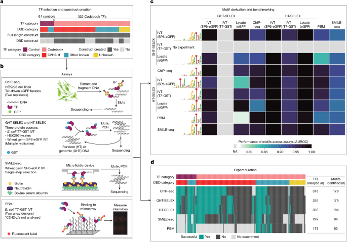
Sequences and accompanying information are given in Supplementary Tables 2–4. In brief, we selected Codebook TFs (and their DBDs) from information published in a previous study¹ and posted at https://humantfs.ccbr.utoronto.ca. Inserts named with a ‘-FL’ suffix correspond to the full-length ORF of a representative isoform of the protein. Those with a ‘-DBD’ suffix contain all of the predicted DBDs in the protein flanked by either 50 amino acids or up to the amino or carboxy terminus of the protein. Those with a ‘-DBD1’, ‘-DBD2’ or ‘-DBD3’ suffix contain a subset of the DBDs present in the proteins; these were manually designed, mainly for large C2H2-zf arrays. Inserts were obtained as recoded synthetic ORFs (BioBasic) flanked by AscI and SbfI sites and subcloned into up to three plasmids: (1) pTH13195, a tetracycline-inducible, N-terminal eGFP-tagged expression vector with FLiP-in recombinase sites⁸; (2) pTH6838, a T7-promoter driven, N-terminal GST-tagged bacterial expression vector⁵³; and (3) pTH16500 (pF3A-ResEnz-egfp), a SP6-promoter driven, N-terminal eGFP-tagged bacterial expression vector, modified from pF3A–eGFP⁷ to contain the two restriction sites after eGFP.

Protein production

Each experiment used a protein expressed from one of the following systems: (1) FLiP-in HEK293 cells (Thermo Fisher Scientific, R78007), induced with doxycycline for 24 h, used for inserts in pTH13195; (2) PURExpress T7 recombinant IVT system (NEB, E6800L), for inserts in pTH6838; or (3) SP6-driven wheat germ extract-based IVT (Promega, L3260), for inserts in pTH16500.

DNA-binding assays

We followed previously described protocols for ChIP–seq⁸, PBMs⁵⁰ and SMiLE-seq⁷. Detailed descriptions of GHT-SELEX, HT-SELEX, ChIP–seq and SMiLE-seq data collection and initial analyses are provided in the accompanying papers^10,11,12,13. For PBMs, we analysed proteins on two different universal PBM arrays (HK and ME), with differing probe sequences⁵⁴, but did not analyse most C2H2-zfs owing to low success rates with this assay, presumably due to long binding sites. By default, we analysed each protein twice by ChIP–seq (with full-length constructs only)¹¹. We analysed each construct by HT-SELEX and GHT-SELEX once by default (that is, as full-length and DBDs), and some constructs were analysed multiple times to examine the impact of experimental variables as the GHT-SELEX method was developed¹⁰. We ran SMiLE-seq assays for 278 TFs, which corresponded to 388 constructs. Controls were omitted given that most were selected because they already had published SMiLE-seq data, which resulted in 299 TFs with SMiLE-seq-derived motifs. A subset of Codebook proteins (mainly those with unknown DBDs) were also omitted owing to lack of success in all other assays. A randomly selected subset of 82 constructs was analysed multiple times to assess reproducibility across SMiLE-seq experiments. Anti-eGFP antibody (Ab290, Abcam) was used as the major antibody across all the assays (ChIP–seq, GHT-SELEX and western blots), with method-specific amounts^10,11. Each ChIP reaction used 2 µl undiluted polyclonal antiserum, corresponding to 10 µg total IgG, immobilized on 60 µl protein G magnetic bead suspension (Dynabead 10004D, ThermoFisher). For HT-SELEX and GHT-SELEX, antibody-bead master mixes were prepared by immobilizing 6 µl antiserum on 100 µl protein G sepharose bead slurry (Cytiva, 28-9670-70), and 1 µl aliquots of the resulting mixture were used for each selection, which corresponded to approximately 0.06 µl antiserum (300 ng total IgG) per reaction. For western blotting, membranes were incubated in 15 ml antibody solution diluted 1:5,000, which corresponded to approximately 15 µg total IgG per membrane.

Data processing and motif derivation

The accompanying paper¹² describes motif derivation and evaluation in detail. In brief, after initial preprocessing, we obtained a set of ‘true positive’ (likely to be bound) sequences for each individual experiment. A total of 721 out of 4,873 experiments were removed at this step owing to a low number of likely bound sequences or to other technical issues, as documented in Supplementary Table 4. We then applied a suite of tools (listed in Supplementary Table 15) to a training subset of the data from each experiment and tested the resulting motifs on a test subset of the data from the same experiment and on the independent data for the same TF (that is, the test sets from all other experiments performed for the same TF). We used a binary classification regimen for all experiments and all motifs and scored the motifs using a variety of criteria, including the area under the receiver operating characteristic curve (AUROC) and the area under the precision–recall curve. The full set of motifs (as PWMs) is available at Zenodo⁵⁵, and an interactive browser is available at https://mex.autosome.org.

Systematic filtering of artefactual motifs

While curating the datasets and assembling a reliable motif collection, we accounted for enrichment of similar artefact motifs. These recurrent DNA patterns were detected owing to systematic experimental noise or peculiarities of particular motif discovery tools. For example, in HT-SELEX experiments, an ACGACG motif was often enriched. This sequence is a presumed artefact as it matches the constant flanking region. In experiments with cell lysates, motifs of abundant native proteins in HEK293 cells were sometimes enriched (for example, NFI, YY1 and ETS-family TFs). To minimize the influence of these artefacts, we performed the following tasks: (1) manually compiled a list of recurrent artefact motifs (Supplementary Table 16); and (2) scanned the entire motif collection with MACRO-APE⁵⁶ and removed motifs that were highly similar to those in our catalogue of artefacts. We also removed motifs that matched the constant, non-variable regions of the DNA used in HT-SELEX, GHT-SELEX and SMiLE-seq experiments. We did not filter out ETS-related motifs for ETS-family positive controls, such as ELF3, FLI1 and GABPA. Subsequent to expert curation, we confirmed that enriched k-mers in HT-SELEX experiments did not correspond to potential artefacts associated with individual expression systems¹⁰.

Evaluation of motif discovery success rate

To estimate the success rate of different motif discovery tools across different platforms, we started with the successful experiments and TFs. For each combination of a platform X (for example, ChIP–seq) and a motif discovery tool Y (for example, Autoseed), we computed the number of experiments (Extended Data Fig. 1c) or TFs (Extended Data Fig. 1d) that produced a motif highly similar to the reference motif (that is, the one manually curated for the TF). For a specific experiment or TF, we took the entire set of candidate motifs generated by that combination of platform X and tool Y and checked whether any of those motifs passed the similarity threshold using a one-pass scan of MACRO-APE (v.3.06)⁵⁶ ScanCollection with the following parameters: -c 0.05 –rough-discretization 10 –precise 100500. Before comparison, the motifs were converted to log-odds PWMs as previously described¹².

Experiment evaluation by expert curation

To gauge the success of individual experiments, we implemented an ‘expert curation’ workflow with an initial voting scheme in which a committee of annotators gauged whether individual experiments should be deemed successful (that is, included in subsequent analyses). All experiments were examined by at least three annotators. A subcommittee (A.J., I.V.K. and T.R.H.) jointly resolved all cases of disagreement among initial annotators (around 300 experiments) and then reviewed all successful experiments. Annotators had access to an early version of the MEX portal (https://mex.autosome.org, as previously described¹²), which contains the results of all PWMs scored against all experiments, and they were tasked with gauging whether the experiments produced PWMs that were similar across experiments or scored highly across experiments. Annotators also considered whether the motif was consistent with those for other members of their protein family (for example, BHLHA9 produced an E-box-like motif, CAnCTG) and/or similar between closely related paralogues (for example, ZXDA, ZXDB and ZXDC all produced similar motifs). We also considered whether (and how many) ‘peaks’ were obtained from ChIP–seq or GHT-SELEX, and whether these peaks were common to independent experiments (for example, both ChIP–seq and GHT-SELEX). Annotators were further given a measure of similarity between Codebook PWMs and any PWMs in the public domain, as well as enrichment of known or suspected common contaminant motifs in any experiment.

Post-evaluation peak processing

After identification of successful experiments, we re-derived peak sets for ChIP–seq and GHT-SELEX experiments to obtain a single peak set for each TF, as described in the accompanying papers^10,11. In brief, for ChIP–seq, we repeated peak calling using MACS2 (v.2.2.9.1)⁵⁷ and experiment-specific background sets using a previously described method⁸, then merged the peak sets for replicates of the same TF with BEDTools (v.2.30.0) merge⁵⁸ (see accompanying manuscript¹¹: ‘ChIP peak replicate analysis and merging’). We derived GHT-SELEX peaks using a new method, MAGIX, that calculates enrichment of reads in each cycle and treats different experiments as independent statistical samples to obtain a single enrichment coefficient per peak¹⁰.

Expert motif curation

For this study, to identify a single representative PWM for each TF, we first compiled a set of the highest-scoring candidate PWMs for each TF (as summarized above and in a previous study¹²), then ran additional tests with them, using the reprocessed peak data, and manually evaluated the outputs. We started with the union of 3 sets of 20 PWMs for each TF: the 20 PWMs with the highest AUROC (as calculated using a previously described method¹²) on any successful ChIP–seq experiment for the given TF, any successful GHT-SELEX experiment for the given TF and any successful HT-SELEX experiment for the given TF. These PWMs were selected regardless of the dataset from which they were derived. We then reassessed these PWMs against ChIP–seq and GHT-SELEX data with two parallel methodologies. First, we recalculated the AUROC for each of the candidate top PWMs on the merged, thresholded sets of ChIP-seq peaks (P < 10⁻¹⁰)¹¹ using AffiMX (v.1)²⁵ to score each peak. We generated negative sets using BEDTools (v.2.30.0) shuffle⁵⁸ with the -noOverlapping option to create sets of random genomic regions with the same number of peaks and with the same peak-width distribution as the corresponding ChIP–seq peak sets. We used the same technique to calculate AUROC values for GHT-SELEX, with thresholded peak sets (using a ‘kneedle’⁵⁹ specificity value of 30 in the sorted enrichment values¹¹). In parallel, we calculated the Jaccard index to measure the overlap between PWM matches (identified using MOODS (v.1.9.4)⁵¹ with -p 0.001) versus ChIP–seq peaks and GHT-SELEX peaks as two separate measures. The overlap in each case was maximized by applying different thresholds on the peak sets and choosing the cutoff at which the Jaccard index was the highest¹⁰. We then applied expert curation (by a committee consisting of A.J., T.R.H., K.U.L., A.F., R.R., M.A. and I.Y.) to choose a single representative PWM with high performance on all compiled scores that, all else being equal, also reflected reasonable expectation from the DBD class (including recognition-code-predicted motifs, see accompanying manuscript¹⁰) and had sufficient IC.

Motif similarity analysis and clustering

We took two different approaches to determine the number of distinct motifs represented by the Codebook TFs and the number of previously unknown motifs added to the human TF repertoire. In the first approach, we identified the similarity between 1,582 PWMs representing the Codebook TFs (177 PWMs, 177 TFs) and TFs with previously known specificities (1,405 PWMs, 1,211 TFs). The Codebook TF PWM set is the set of representative PWMs for the 177 Codebook proteins with identified motifs. For TFs with previously known specificities, the set of PWMs identified as the ‘best’ in a previous study¹ was used, except for two TFs (MTF2 and PHF1) that did not have an assigned PWM. For these two TFs, the PWMs were retrieved from CisBP⁵³. We used the correlation between pairwise affinities to 150,000 random sequences of length 100, as calculated using MoSBAT (v.1)²⁵, as the metric for PWM similarity. We then clustered the 177 Codebook TFs on the basis of these PWM similarities with PCC and average linkage and identified the ideal number of clusters (129) by determining the optimal silhouette value⁵² using the silhouette function from the ‘cluster’ package (v.2.1.8.1) in R (v.4.3.2), which corresponded to splitting PWMs into clusters at a distance of 0.76. We then clustered the entire set of 1,582 motifs and used the same distance to split the PWMs into clusters. This process resulted in 613 clusters, 92 of which contained only Codebook TFs. The set of motifs used in the clustering and their cluster membership are provided in Supplementary Table 10.

Independently, and to obtain a non-redundant set of motifs for MARA analysis, we followed a previously described procedure⁶⁰, but with the addition of Codebook motifs. First, we merged HOCOMOCO (v.12)²⁹ motifs with those evaluated in Codebook, preferably selecting those built with ChIPMunk and ranking high in benchmarking¹² to maintain consistency with HOCOMOCO (v.12), which was fully built with ChIPMunk. Having the joint motif collection, we estimated the motif similarities with MACRO-APE (v.3.0.6)⁵⁶ at the motif P value cutoff of 0.0005 and a default matrix discretization parameter (-d) of 1 (increased to 10 for improved precision only for motif pairs with the Jaccard similarity over 0.01 at -d 1). Next, using the pairwise motif similarity matrix, we performed agglomerative clustering (‘average’ linkage) with sklearn (v.1.8.0). The number of clusters was taken to maximize the silhouette score. Clusters of low-quality motifs (HOCOMOCO ‘D’) were discarded. Finally, for each cluster, a single representative motif was taken according to the highest average similarity to all other motifs in the cluster. The non-redundant set of representative motifs is available for download from Zenodo⁶¹, and the motif clusters annotation is available in Supplementary Table 11.

Motif degeneracy analysis

To explore whether low IC is an intrinsic feature of some binding motifs, we adjusted the IC of PWMs and tested the prediction accuracy of ChIP–seq and GHT-SELEX binding sites. PWM IC was adjusted on a per-base-pair basis by iteratively scaling probabilities for each base at each position until the PWM reached an average IC of 1 bit per base pair. The script ‘logo_rescale.pl’ is available at GitLab (https://gitlab.sib.swiss/EPD/pwmscan).

Comparison to external peak sets and PWMs

For comparison, we downloaded ChIP–seq peak sets from GTRD⁶² and ENCODE (4.12.2023)⁶³ for all Codebook TFs. We then divided these data into four categories corresponding to the cell type: HEK293/HEK293T, HepG2, K562 and other cells. We preferentially selected the peak sets from GTRD because GTRD has processed the majority of ENCODE consortium experiments, together with many non-ENCODE experiments. When multiple experiments were available for a TF in a cell-type category, we selected the experiment with higher peak counts. If multiple computational methods had been used to derive peak sets for the selected experiment, we chose the peak set using a preferential order of MACS, GEM, SISSRS, PICS and PEAKZILLA. See Supplementary Table 7 for identifiers and metadata of the reference datasets.

For PWM scoring, the external peak sets were used as downloaded, with the exception of peak sets that were generated with the GEM peak caller, which have a peak width of 1 (summit only), and were therefore expanded 250 bases in both directions. For Codebook data, we used the merged and thresholded Codebook ChIP–seq peak sets as in ‘Expert motif curation’. We generated negative peak sets using BEDTools (v.2.30.0) shuffle⁵⁸ with the -noOverlapping option to create sets of random genomic regions with the same number of peaks and the same peak width distribution as the corresponding ChIP–seq peak sets. We downloaded PWMs for all Codebook TFs from JASPAR (2024 version)⁶⁴, HOCOMOCO (v.12)²⁹ and Factorbook⁶⁵ (downloaded 15 December 2023) (Supplementary Table 13). We scanned Codebook and external peak sets (and corresponding negative sets) with the representative (that is, expert-curated) Codebook motifs (PWMs) using AffiMX (v.1)²⁵ and calculated AUROC values. Furthermore, for the 20 Codebook TFs with a successful Codebook ChIP–seq experiment, a Codebook PWM, an external ChIP–seq experiment and an external PWM, we compared the performance of PWMs across the different peak sets as follows. We first selected a single external PWM for each of the 20 TFs by scanning each PWM for a given TF on each external peak set for the same TF and identifying the PWM that produced the highest AUROC. We then used these highest scoring PWMs to scan the corresponding Codebook data and to calculate AUROC values.

Curation of external motifs for previously uncharacterized TFs

For this analysis, we considered all proteins that were previously annotated as putative TFs¹ but did not, at that time, have a credible motif. We downloaded all motifs for these TFs from JASPAR (2024 version)⁶⁴, HOCOMOCO (v.12)²⁹ and Factorbook⁶⁵ (downloaded 15 December 2023), which resulted in a set of 484 PWMs that we then manually assessed with the following considerations: (1) whether similar motifs were obtained for the protein from multiple independent datasets; (2) whether the motif was consistent with the structural class of the TF and; (3) whether the motif was likely to describe the inherent specificity of the protein and not, for example, reflect a target site of another TF or a probable artefact. The curated motifs are listed in Supplementary Table 13 with more details in Supplementary Table 10. The PWMs themselves are available in Supplementary Data 1, and examples of artefactual and correct external motifs are shown in Extended Data Fig. 10.

Identifying and scoring promoter sequences for MARA

MARA requires promoter activity (gene expression) data across samples and motif scores across promoters. The former was downloaded from the FANTOM5 web resource (https://fantom.gsc.riken.jp/5/), hg38_fair+new_CAGE_peaks_phase1and2_tpm_ann.osc.txt, log₂-transformed with a pseudocount of 0.05 and filtered, leaving only promoters of genes encoded in the nuclear genome and removing time courses, perturbations and human total RNA samples. This process resulted in 209,374 individual promoters and 1,020 samples (including replicates) that belonged to 583 unique samples (142 tissues, 187 primary cells and 254 cell lines; Supplementary Table 12 and Zenodo⁶¹). Motif scanning was performed on regions from FANTOM5 hg38_fair+new_CAGE_peaks_phase1and2.bed, taking 250 bp upstream and 10 bp downstream from the representative TSS position as indicated in FANTOM5 data. Next, we used SPRY-SARUS (v.2.2.3; https://github.com/autosome-ru/sarus) to compute the sum-occupancy scores⁶⁶ for each representative motif of the motif clusters (see the section ‘Motif similarity analysis and clustering’). The final analysis was performed with 632 motif clusters (130 clusters containing only Codebook motifs, 471 clusters of known motifs and 31 mixed clusters) corresponding to TFs that were jointly expressed >0 in at least one of the FANTOM5 samples.

For MARA, we used MARADONER (v.0.13)⁶⁷, a command-line tool written in Python and available in the PyPi repository. The analysis was performed using maradoner create, maradoner fit and maradoner export with default parameters (https://github.com/autosome-ru/MARADONER).

Conceptually, MARADONER extends the original logic of MARA³⁶ and isMARA⁶⁸. The basic assumption is that the promoter activity in each sample is a linear function of sample-specific motif activities, for which each motif represents a set of TFs with shared binding specificity. We used the following matrix-variate linear mixed model:

where Y is a matrix of promoter activity in log-scale of shape p × s (where p is the number of promoters and s is the total number of samples), μ_p and μ_s are promoter-wise and sample-wise means, respectively, 1_n is a vector of ones of length n, B is a matrix of promoter-level motif scores of shape p × m, U is a random matrix of motif activities of shape m × s, E is a random error/noise matrix of shape p × s, MN is a matrix-variate normal distribution, I_p is an identity matrix of shape p × p, D is a diagonal matrix of noise variances of shape s × s, Σ is a m × m matrix of motif variances, G is a diagonal s × s sample-wise scaling matrix, and μ_m is a motif-wise mean vector of motif activities. In contrast to the classical MARA, modelling μ_m allows explicitly distinguishing activators from repressors. The number of unique parameters in each of the diagonal matrices D and G is equal to g (the number of groups, in our case, the number of unique samples excluding replicates), which is less than s (the total number of samples), which enables an increase in certainty in the parameter estimates of D, G.

MARADONER performs estimation via a four-stage restricted maximum likelihood procedure. First, we isolate parameters in E by finding a transformation that is orthogonal to the 1_p, 1_s, B matrices, which enables us to focus on estimating D solely. Second, we find a transformation that is orthogonal only to the 1_p, 1_s vectors. This makes estimating parameters in Σ, G possible given the known parameters in D. Third, we find a transformation that is orthogonal to B only, and we estimate the total mean effect of the \({{{\boldsymbol{\mu }}}_{{p}}{{\bf{1}}}_{{s}}}^{{\rm{T}}}+{{\bf{1}}}_{{p}}{{\boldsymbol{\mu }}}_{{s}}\) term. Finally, given the knowledge of all other parameters, we estimate the mean motif activity vector µ_m. Then, if we disentangle U from \(B{{{\boldsymbol{\mu }}}_{{\rm{m}}}{{\bf{1}}}_{{s}}}^{{\rm{T}}}\), the deviation from motif mean matrix \(\hat{U}=U-B{{{\boldsymbol{\mu }}}_{{\rm{m}}}{{\bf{1}}}_{{s}}}^{{\rm{T}}}\) can be interpreted as a sample-specific variation in motif activity. \(\hat{U}\) is then obtained as a maximum a posteriori estimate. Alongside ‘raw’ maximum a posteriori estimates of \(\hat{U}\) for downstream analysis, MARADONER also reports standardized motif activities, which are obtained by dividing each motif activity by the square root of its posterior variance.

The availability of the maximum likelihood estimates of motif-specific variances allows for an ANOVA-like test using the asymptotic properties of maximum likelihood estimate for each motif. To this end, MARADONER performs the Wald test by extracting by square root of the diagonal entries from the asymptotic covariance matrix of parameter estimates that correspond to elements from Σ (the standard errors).

MARADONER assumes that the gene expression (or promoter activity, in the case of FANTOM5 CAGE data) is provided in the log-scale. As for the motif-scores matrix B, by default, each column is normalized by taking the negative logarithm of its empirical survival function.

TOP and CTOP peak set analyses

To obtain the TOP sites, we first identified thresholds for ChIP–seq peaks, GHT–SELEX peaks and PWM-derived ‘peaks’ (see below) that maximize the three-way Jaccard metric (overlap or union) of the three sets, with the thresholds calculated for each TF independently. We converted PWM matches (derived using MOODS (v.1.9.4)⁵¹ using a P value cutoff of 0.001) into peaks by merging neighbouring matches with a distance less than 200 bp and re-scoring them using the sum-occupancy for clusters. We then identified TOPs as peaks exceeding these thresholds in all three sets and overlap in all three. To obtain the CTOP sites, we then extracted phyloP scores from the Zoonomia consortium⁶⁹ for each base at each TOP site (and 100 flanking bases), removed sites overlapping the ENCODE Blacklist⁷⁰ or protein-coding sequences (owing to the skew in phyloP scores caused by codons) and applied three different statistical tests for significance of phyloP scores over the PWM match: two that tested association between the IC and the phyloP value at each base position of the PWM (using either PCC or likelihood-ratio test), and one that tested for higher phyloP scores over the PWM match (Wilcoxon test). Greater detail on these specific operations is given in the accompanying manuscripts^10,11, and the custom R (v.4) script for is available at GitHub (https://github.com/imyellan/Codebook_CTOP_scripts).

Intersection of TOPs and CTOPs and genomic features

We first clustered all CTOPs using BEDTools (v.2.30.0) merge⁵⁸, with a maximum distance of 100 bp, then intersected them with the following genomic feature sets: basic canonical protein-coding promoters from GENCODE (v.44)⁷¹, defined as 1000 bp upstream and 500 bp downstream of the canonical TSS; the ‘unmasked CpG island’ track, PhastCons Conserved Elements from the Multiz 470 Mammalian alignment, and RepeatMasker track from UCSC⁷²; and ChromHMM HEK293 enhancers¹¹. We classified promoters as CpG island or non-CpG island on the basis of the GENCODE basic TSS being within ±50 bp of a CpG island from the unmasked track. We classified the CTOP clusters as associated with a single type of genomic feature in the following order of priority: CpG island associated with a protein coding promoter; other CpG islands; a non-CpG island-associated protein-coding promoter; an enhancer; clusters containing a CTCF-binding site but not overlapping a CpG island, promoter or enhancer; overlapping a transposable element and none of the previous categories; overlapping a non-transposable-element repeat and none of the previous categories; and ‘other’ for CTOP clusters not intersecting any examined features.

Analysis of ASB

We reasoned that the GHT-SELEX and ChIP–seq experiments facilitate direct assessment of ASB of TFs by quantifying the allelic imbalance of read counts at SNVs. We note that the data were not initially intended for this purpose, and caveats include relatively low read counts, linked SNVs and the fact that HEK293 cells have an abnormal karyotype and this cell line was derived from a single individual. Nonetheless, SNV calling (see below) produced 924,997 variant calls overlapping with dbSNP common SNPs (889,814 variant calls from 361 ChIP–seq experiments and 35,183 from 370 GHT-SELEX multicycle experiments) at 122,364 unique genomic locations (corresponding to distinct rsSNP IDs). Of these, 10,009 SNPs corresponded to 12,060 ASBs of 152 Codebook TFs and 39 positive controls. That is, there was a significant imbalance in the number of sequencing reads supporting the reference or the alternative SNP alleles in ChIP–seq (10,575 ASBs) or GHT-SELEX (1,485 ASBs) read alignment (Extended Data Fig. 5 and Supplementary Table 8). SNP calls and ASBs are available at Zenodo⁷³ (https://doi.org/10.5281/zenodo.18224872).

Variant calling

For variant calling directly from ChIP–seq and GHT-SELEX data, we started by mapping raw ChIP–seq and pre-trimmed GHT-SELEX reads¹² to the hg38 human genome assembly using bwa-mem (v.0.7.1) with default settings (Extended Data Fig. 5a). Next, we used filter_reads.py (originally taken from stampipes (https://github.com/StamLab/stampipes/tree/encode-release), accessed September 2022) to filter out reads with >2 mismatches and mapping quality <10. Then we followed a previously described workflow²¹ for SNV calling and read counting (https://github.com/autosome-ru/MixALime/tree/main/natcomm_supp_scripts, accessed December 2025):

1. 1)

   samtools reheader (v.1.16.1) was used to set the identical sample SM field in all alignment files;

2. 2)

   SNP calling was performed using bcftools mpileup (v.1.10.2)⁷⁴ with –redo-BAQ –adjust-MQ 50 –gap-frac 0.05 –max-depth 10000 and bcftools call with –keep-alts –multiallelic-caller;

3. 3)

   the resulting SNPs were split into biallelic records using bcftools norm with –check-ref x -m – followed by filtering with bcftools filter -i “QUAL>=10 & FORMAT/GQ>=20 & FORMAT/DP>=10” –SnpGap 3 –IndelGap 10 and bcftools view -m2 -M2 -v snps leaving only biallelic SNPs covered by 10 or more reads;

4. 4)

   SNPs were annotated using bcftools annotate with –columns ID,CAF,TOPMED and dbSNP (v.151)⁷⁵;

5. 5)

   heterozygous variants located on the reference chromosomes with genotype quality (GQ) ≥ 20, depth ≥ 10 and allelic counts ≥ 5 on each allele were filtered with awk (v.5.0.1);

6. 6)

   WASP (v.0.3.4)⁷⁶ was used with bwa-mem and filter_reads.py to account for reference mapping bias;

7. 7)

   count_tags_pileup_new.py (edited version of the original script count_tags_pileup.py from GitHib (https://github.com/vierstralab/nf-allelic-mapping/tree/main/bin), which was adapted by removing the settings related to DNase-seq specifics) was used to obtain allelic read counts with pysam (v.0.20.0);

8. 8)

   recode_vcf.py was used to convert the resulting BED files to VCF.

Of note, triallelic SNVs were split into two biallelic records.

ASB calling and annotation

ASB calling was performed independently for GHT-SELEX and ChIP–seq data. To account for aneuploidy and copy-number variation, the profiles of relative background allelic dosage were reconstructed with BABACHI (v.2.0.26) using default settings⁷⁷ (abstract O3). The allelic imbalance was estimated with MIXALIME (v.2.14.17)²¹, starting with mixalime create. Next, we fitted a marginalized compound negative binomial model (MCNB) using mixalime fit specifying MCNB and setting –window-size to 1,000 and 10,000 for GHT-SELEX and ChIP–seq, respectively, taking into account lower coverage and fewer SNPs called from GHT-SELEX. Finally, we used mixalime test followed by TF-wise mixalime combine to obtain the TF-specific ASB calls. This process resulted in 12,060 identified ASBs at 5% FDR (corrected for multiple tested SNPs).

Technically, the GQ of SNPs and ASBs was much higher than the default threshold, and most of the ASB SNPs were supported by two or more datasets (Extended Data Fig. 5d,e).

We then identified 3,564 ASBs that overlapped a PWM hit (P < 0.001) for the associated TF. Of note, ASBs that did not overlap a PWM hit may be marker variants acting indirectly by being linked to ‘causative’ SNVs. For ASBs with PWM hits, we calculated the PWM scores for both alleles and estimated the right-tailed P values of those scores against a uniform background distribution using PERFECTOS-APE (v.3.0.6)⁷⁸. The fold change between uncorrected alternative (Alt) and reference (Ref) allele P values, log₂[Alt/Ref], reflected the PWM-predicted allelic preferences, with positive or negative values reflecting the preference for the Alt or Ref allele, respectively. ASBs with an absolute log₂[fold change] > 1 were labelled as ‘motif concordant’ or ‘motif discordant’, depending on whether the allelic preference exhibited by the greater ChIP–seq or GHT-SELEX read coverage (Ref > Alt or Alt > Ref) was consistent with the difference in the respective PWM scores (Extended Data Fig. 5c).

To globally support the relevance of the Codebook ASB calls, we obtained a joint set of 22,064 ASBs by running MIXALIME (v.2.28.0) multiple_combine for joint aggregation of the allelic imbalance P values over all processed datasets (Supplementary Table 9). Next, for the resulting joint set of ASB–SNPs, we estimated the significance of the overlap with GTEx (v.8)²⁴, ADASTRA (v.6.1)²² and EBI GWAS Catalog (v.1, e115_r2025-12-03_full)²³ using two-sided Fisher’s exact test.

Reporting summary

Further information on research design is available in the Nature Portfolio Reporting Summary linked to this article.