A global molecular code for birth order and neuronal identity in Drosophila

scRNA-seq data generation

To discriminate technical from biological variability, we used flies from different genetic backgrounds^19,77, enabling us to generate scRNA-seq libraries of VNCs of different sex and developmental stages and separate them after sequencing through single-nucleotide polymorphisms (SNP)-based sample demultiplexing (see below)⁷⁸ (Extended Data Fig. 1). Randomized samples from different genotypes were used for the same sex and developmental stages across experiments. In total, data were collected from 92 individual animals, covering four developmental stages and both sexes. Each stage–sex condition is represented by 5 to 18 biological replicates, covering between 5 and 11 different genotypes. Some experimental preparations were used to create 2 or 3 independent libraries.

Dissociation

For each stage–sex condition, several genotypes and individuals were used, as summarized in Supplementary Table 1. Flies of the genotypes indicated in Supplementary Table 2 were allowed to mate and their larvae developed at 25 °C until white pupae stage. Then pupae were collected with forceps, sexed under a dissecting scope and put in either male or female vials to develop until the correct stage, that is, 6, 24, 36 or 48 h.a.p.f. VNCs were dissected in ice-cold DPBS (Dulbecco’s PBS, Gibco). A maximum of 8 VNCs, each of a different genotype, was pooled in a low-bind Eppendorf tube containing 100 µl of DPBS on ice. VNCs from animals of two or three different developmental stages and sex were pulled in the same tube (6 + 24 h.a.p.f., 24 + 48 h.a.p.f. or 24 + 36 + 48 h.a.p.f.). Four brain samples were included in the last round of experiments, but later excluded from the analysis of VNC. After dissections, tissues were collected at the bottom of the tube by centrifugation (800g, 5 min, 4 °C), DPBS was replaced with 50 µl of dispase I (3 mg ml⁻¹, Sigma-Aldrich, D4818, reconstituted in 50 mM HEPES/KOH pH 7.4, 150 mM NaCl) and 75 µl of collagenase I (100 mg ml⁻¹, Invitrogen, 17100-017, reconstituted in HBSS). VNCs were dissociated in a thermo mixer (Eppendorf) at 25 °C at 500 rpm for 30 (6 + 24 h.a.p.f. samples) or 40 min (24 + 36 + 48 h.a.p.f. samples). Dissociation was aided by pipetting up and down 10 times every 10 min ensuring that the tip touched the bottom of the tube to increase the mechanical stress. Dissociated cells were centrifuged (800g, 5 min, 4 °C), washed once with DPBS and resuspended in 180 µl of DPBS with 0.04% BSA. The cell suspension was filtered through a 10 µm filter (pluriStrainer, Cambridge Bioscience, 43-50010-03). Viability, presence of debris and cell number were accessed using the Countess II automated cell counter (Invitrogen).

Library preparation and sequencing

Samples were collected on 3 different days. Each day, a total of 4 different cell suspensions (independent samples) was generated, each containing different combinations of genotypes, ages and sex. Single-cell expression libraries were generated at the CRUK-CI sequencing facility using Chromium Next GEM Single Cell 3′ HT v3.1. We aimed to load each sample in duplicate, 20,000 cells per lane. Before sequencing, libraries were inspected on the TapeStation. Sequencing was performed on the NovaSeq6000 machine (Illumina) with the following sequencing parameters: 28 regular cycles of which 16 are 10x barcode and 12 are unique molecular index, 10 i7-index cycles, 10 i5-index cycles, 90 regular cycles.

scRNA-seq data processing

No formal experimental blinding was applied for the generation and analysis of the scRNA-seq atlas; however, computational analyses were performed in an unsupervised manner, and clustering and dimensionality reduction were performed without using sample identity.

CellRanger

Data from the NovaSeq6000 sequencer were processed using CellRanger v.8.0.0 using the cellranger count function with the default parameters. CellRanger reference index genome was built on genome assembly BDGP6.32 supplemented with the coding sequences for the expected transgenes (Supplementary Table 6). Before quality control, cell ranger total output was 805,970 cells. The median sample number of reads per cell was 39,142, the number of detected genes per cell 1,511 (min = 183, max = 8,543) and the median number of unique molecular identifiers (UMIs) per cell 4,893 (min = 666, max = 847,868).

Demultiplexing

The output from CellRanger was demultiplexed using applications from the Demuxafy docker container v.3 (https://demultiplexing-doublet-detecting-docs.readthedocs.io/en/latest/index.html)⁷⁹. SNP information for all sequencing reads (Pileups) were generated using cellsnp-lite (v.1.2.3) with the parameters ‘–chrom 2 L,2 R -p 22 –minMAF 0.1 –minCOUNT 100’. Out of the 4 fly chromosomes, only chromosome 2 was used for demultiplexing because, in our cross schemes, it always comes from the DGRP lines, while the remaining chromosomes originate on the other stocks. The demultiplexing package Vireo^78,79 was run twice on the pileups, once using a variant call format (VCF) reference file and once without it (withVCF and noVCF in Extended Data Fig. 1). The VCF file for the first run was generated using the DGRP SNP data from the Aerts laboratory (https://resources.aertslab.org/DGRP2/NCSU/final/dm6/DGRP2.source_NCSU.dm6.final.SNPs_only.vcf.gz). The parameters used were ‘-N noSamples -p 4 –randSeed=1’ where noSamples is the number of different genotypes present in the given sample. The noVCF run can identify all genotypes in an unbiased way but does not provide the identity of the groups, that is, while it produces groups 1 to 7, it does not indicate which genotype each group corresponds to. Conversely, the run withVCF can identify most genotypes but is less efficient in identifying singlets due to the variable quality of VCF information across DGRP genotypes and the confounding effect introduced by DGRP heterozygosity of chromosome 2 (only one parent carried the DGRP chromosome). To use the demultiplexing results of the more efficient noVCF runs, we used several source of information to assign groups to genotypes: (1) the correspondence between expected sex and roX1 expression; (2) expression of GFP transgenes; and (3) comparison of the results from noVCF and withVCF Vireo results (Extended Data Fig. 1). In the rare cases in which the genotype assignment provided by the withVCF run disagreed with the sex or GFP transgene expression, these took precedence. Besides enabling assignment of metadata information such as sex and stage of the cell, demultiplexing also enabled removal of doublets, given that those cells have a high fraction of SNPs coming from different DGRP lines. Cells were considered doublets if they were classified as such in the Vireo noVCF run and excluded from further analysis.

Gene annotations

The list of TFs comprises the union of genes annotated as TFs in flybase and TFs reported previously⁸⁰. Annotation of cell surface molecules was taken from ref. ⁸⁰. Genes involved in cellular energy production and stress response correspond to the union of flybase gene lists: CYTOCHROME_C; ELECTRON_TRANSFER_FLAVOPROTEINS; MITOCHONDRIAL_COMPLEX_III; MITOCHONDRIAL_COMPLEX_II; MITOCHONDRIAL_COMPLEX_IV_CYTOCHROME_C_OXIDASE_SUBUNITS; MITOCHONDRIAL_COMPLEX_I_SUBUNITS; MITOCHONDRIAL_COMPLEX_V_ATP_SYNTHASE_COMPLEX_SUBUNITS; heat_shock_prot.

Quality control

The Cell ranger output was imported into an R object using sequentially the functions Read10X and CreateSeuratObject from the Seurat package (v.4)⁸¹ with the default parameters. Some of the last analyses were performed using Seurat (v.5)⁸². A first quality-control filter was applied to exclude cells with fewer than 700 features, more than 20% of mitochondrial genes and more than 50% of ribosomal genes. Genes expressed by fewer than three cells in the dataset were also excluded. Samples showed a bimodal distribution of UMIs and features across cells, except for SITTD8, for which the distribution was unimodal. For this reason, we excluded SITTD8 from further analysis.

Data integration

Data integration was performed twice following the same pipeline (see below) to integrate the full dataset (including neurons and glia) as well as the subsets containing either neurons or glia.

Data integration was performed using the rpca algorithm in Seurat. In brief, 3,000 features were found using SelectIntegrationFeatures, FindIntegrationAnchors was then run on those features using the 24 h.a.p.f samples as reference and lastly, the anchors were used with the IntegrateData function with a k.weight = 100 (or number of cells −2 for small samples). This integration process removes variability due to stage and genotype. Cells with fewer than 3,000 UMIs or in clusters with an average number of UMIs smaller than 3,000 were excluded from further analysis as these were deemed to be low quality. The resulting VNC dataset has a median of 23,976.3 UMIs (min = 3,000, max = 565,460) and a median number of genes of 3,445 (min = 731, max = 8,428).

Atlas annotation

Neurons and glia

To annotate neurons and glia we calculated, using the Seurat function AddModScores, enrichment scores for glial (wrapper, repo, CIC-a, loco, CG10702, CG6126, Gs2, Egfr, Tret1-1, bdl, Zasp52, rols, ine, CG5404, CG14688, CG31663, ry, CG4752, betaTub97EF, CG32473, LManII, Eaat1, alrm, Eaat2, axo, Vmat, moody, Indy, zyd), neuronal (elav, nSyb) or ‘other’ (CG11835, alphaTub85E, Act57B, betaTub60D, CG5080) marker genes. Markers for the category ‘other’ were chosen for being specifically expressed in a cell population lacking neuronal as well as glial markers. Gene Ontology analysis identified several genes enriched in cells of mesenchymal origin among markers for the other category. Categorical assignment of cells to glia, neuron or other was done based on a cluster-based winner-takes-all criterion. The category ‘other’ was excluded from any further analysis.

Glia types

Glial clusters were annotated according to the expression of previously reported markers⁸³. Specifically sim expression was used for midline glia, CG6126 for MAP, ltl for subperineurial, alrm and Tre1 for astrocytes, wrapper for cortical and axo for ensheathing glia. Similarly to neurons and glia, glial identity was assigned based on a cluster-based winner-takes-all criterion.

Neurogenesis wave and maturation state

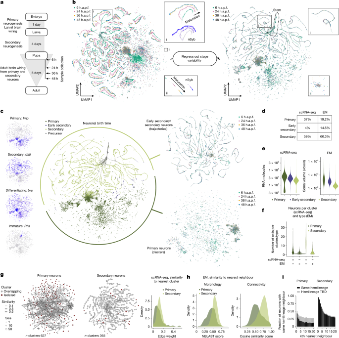
The adult brain contains primary neurons, born in the embryonic phase, and secondary neurons, born during larval stages. To identify these distinct populations in our atlas, we used the markers Imp (primary) and dati (secondary)^30,60,84. First we assigned categorical identity to neurons expressing high levels of markers (primary, Imp > 2; secondary, dati > 2 in the stage-integrated data slot), producing nearly completely mutually exclusive labels. We reasoned that neurogenesis wave information might be more prominent in earlier developmental stages and used the obtained labels to train a classifier using the devCellPy machine learning framework⁸⁵ with parameter rejCutoff = 0.5 and testSplit = 0.1. The trained model was used to predict primary and secondary labels across the atlas. Expression data for training and classification included all 3,000 genes from the stage-integrated data slot.

The stem region of our atlas contains cells with low expression of dati and markers of mature neurons, such as brp and nSyb, and it is devoid of 36 h.a.p.f. and 48 h.a.p.f. cells, suggesting it corresponds to neuronal precursors. We annotated these neurons using a similar strategy as above, but using brp (>1.5) for mature neurons and the chromatin remodelling factor Phs (>1.5) for immature ones. Similarly to the neurogenesis wave, we trained the classifier on 6 h.a.p.f. data and then used the model to predict labels across the atlas. In both cases, training and prediction were performed 50 times starting from the same training set and the consensus result was used for the final assignment.

Cell cycle phase

Cell cycle annotation was done using the Seurat function CellCycleScoring. Marker genes for the different phases of cell cycle were obtained from ref. ⁸⁶.

Neurotransmitter identity

Each neuron in the atlas was assigned a fast neurotransmitter identity based on the highest expression level among the markers VAChT (cholinergic), Gad1 (GABAergic) and VGlut (glutamatergic). Neurons were assigned a monoamine class (tyraminergic, octopaminergic, dopaminergic, serotonergic and histaminergic) if they co-expressed the vesicular monoamine transporter (Vmat) and monoamine-specific markers (tyramine: Tdc2⁺, Tbh⁻; octopamine: Tdc2, Tbh; dopamine: Ddc, ple; serotonin: Trh, Ddc; histamine: Hdc).

Hemilineage

To provide experimental evidence for hemilineage assignments, we included among the sequenced samples transgenic lines in which GFP expression is specifically driven in lineages/hemilineages (09A, 01+10B, 07B, 08B+09B). This was obtained either through split-GAL4 intersectional approach (09A, line 1, Dr-AD/Gad1-DBD; 08B + a subset of neurons from 09B, line 4, Lim3-DBD/c15-AD)^35,87,88 or through an immortalization-based strategy (01+10B, line 2, R16A05-AD;R28H10-DBD; 07B, line 3, Dbx-DBD/ey-AD)^31,89.

Annotation of hemilineages was performed using a stepwise approach, integrating information from multiple published and unpublished sources (summarized in Supplementary Table 4). We first assigned hemilineages with strong supporting evidence from previous studies, which helped to reduce the number of unassigned orphan hemilineages requiring further annotation. We started by mapping the adult VNC atlas²⁶ onto the neuronal subset of the developmental dataset and transferring the existing hemilineage annotations to the pupal dataset using the Seurat functions FindTransferAnchors and TransferData with 3,000 variable features and 200 principal components. Then, selectively in secondary neurons, we expanded adult-derived annotation by taking an iterative cluster-based approach. Hemilineage labels were expanded to all cells within a cluster if more than 50% of its neurons were already annotated with the same hemilineage. This procedure was performed iteratively, from high clustering resolution, that is, small clusters, to low clustering resolution, that is, big clusters. Annotations were then discarded if, after the iterative procedure, they accounted for less than 20% of a cluster at an intermediate clustering resolution (resolution = 1.2). Finally, we applied a winner-takes-all strategy when the annotation represented at least 30% of the cluster at a high clustering resolution (resolution = 20). We then resolved ambiguous hemilineage identities in cases in which the adult annotation grouped two hemilineages together, but our dataset showed them as clearly separated clusters (for example, 05B/06B). We calculated DEGs between the two ambiguous clusters using FindMarkers, which confirmed cluster-specific genes and assigned cluster identity according to the relative expected hemilineage size in MANC². For most hemilineages, identity was further corroborated by previously published split-GAL4 lines with experimentally validated expression patterns³⁵ (Supplementary Table 4). We next annotated hemilineages not covered in the ref. ²⁶ adult dataset, but expected to contain more than ten secondary neurons based on the MANC annotation. For this, we combined evidence from neurotransmitter gene expression, GFP expression from reporter lines, markers from the literature^31,80,84, and comparison between cluster size and number of neurons expected based on electron microscopy (EM) data. Iteratively we reclustered only neurons without hemilineage annotation and assigned them to a specific hemilineage based on the expression of identified new markers. A detailed hemilineage-by-hemilineage summary of the annotation strategy used is provided in Supplementary Table 4. This led to an initial assignment of 48 h.a.p.f. secondary neurons. Annotations were discarded if they accounted for less than 30% of a cluster at an intermediate clustering resolution (resolution = 1.2). This led to the identification of high-confidence assignments (Fig. 2c) in 48 h.a.p.f. secondary neurons that were used to train a classifier using the devCellPy machine-learning framework⁸⁵ with the parameters rejCutoff = 0.5 and testSplit = 0.1. The trained model was used to predict hemilineage labels across the atlas at all stages and expanding to primary neurons, using rejCutoff = 0.3 for prediction. Expression data for training and classification included all 3,000 genes from the stage-integrated data slot. Training and prediction was performed 50 times starting from the same training set and the consensus result was used for the final assignment.

Note that, as secondary neurons of hemilineage 15B are exclusively motor neurons, lineage propagation to primary neurons resulted in the broad assignment of 15B identity to all motor neurons, which share many molecular features. Primary 15B neurons are to be intended more broadly motor neurons.

Suboesophageal zone specific hemilineage 27X and 03A in the labium (glutamatergic in contrast to VNC homologues) were assigned based on expression of eya³¹ and fd96Cb, respectively. fd96Cb (CG11922) is associated with the GMR line R74D11 that drives specific expression in one hemilineage in the labium⁹⁰.

Soma segment

We annotated soma segments based on Hox genes known to be expressed differentially along the VNC anterior–posterior axis (Dfd, Scr, Antp, Ubx, abd-A and Abd-B). Hemilineage-specific thresholds were needed because Antp and Ubx antibody staining in L3 larvae revealed a more complex expression landscape than expected by the canonical view (Supplementary Table 7). For example, Ubx protein levels were medium in T2 and high in T3 for 03B, but medium in T3 and high in A in 07B, reflecting expression level differences detected in the atlas³⁷ (Fig. 3a,b, Methods and Extended Data Fig. 4b,c). Dfd⁺ and Scr⁺ cells belong to hemilineages originating in the gnathal ganglia (labial, maxillary and mandibular)⁹¹. Their presence at 6 h.a.p.f. in our dataset probably reflects imprecise excision of the VNC from the brain at this early timepoint when the neck constriction has yet not formed (Extended Data Fig. 4). We assigned all Dfd⁺ or Scr⁺ cells to GNG⁹¹. In those cases in which we had information about hemilineage-specific expression of Dfd and Scr in the different GNGs, we refined annotation (that is, 03B). A more detailed annotation of the GNG segments will be covered in a different manuscript (in preparation). All abd-A⁺ or Abd-B⁺ cells were annotated as A regardless of the developmental stage given that those markers are not expressed outside the abdominal segments. For the annotation of T1, T2, T3 and abdominal cells not expressing abd-A or Abd-B, instead, we first annotated cells at 48 h.a.p.f. and then transferred the annotation to earlier timepoints, due to substantial variation of Antp expression across pupal stages. As the expression pattern of Antp and Ubx is hemilineage specific, we treated each hemilineage independently. In cases in which immunostaining data from L3 larvae indicated that expression of Antp and Ubx genes deviated from the canonical model, we used these data as guidance. A summary of Hox gene expression derived by these data is reported in Supplementary Table 7; specific images are available on request. The workflow followed to annotate soma segments is shown in Fig. 3b. For each hemilineage, we generated violin plots showing expression by cluster at a high clustering resolution for Antp, Ubx and abd-A. These plots helped to choose expression thresholds to assign cells to T1, T2, T3 or A, a critical task when the difference between the different segments is dictated by the level of expression and not by the quality of the gene expressed. Thresholds used for each hemilineage are summaries in Supplementary Table 7. Thresholding based annotation was used as input for further annotation using devCellPy. Cells were excluded from the training set if their assigned label represented less than 10% of the total cells in their cluster. To prevent overtraining, only half of the labelled cells were used to train the classifier. Multilayered classification provides hemilineage-specific soma segment models which are essential to capture the hemilineage-specific Hox gene expression differences. Stage integrated expression values were used to account for expression differences due to developmental stage and allowed transfer of the model learnt using 48 h.a.p.f. data to earlier stages (as done to assign hemilineage identity). The training parameters used were: rejCutoff = 0.5, testSplit = 0.1. The obtained classifier was used to predict the full dataset with prediction parameters: rejCutoff = 0.3. Training and prediction were run 50 times starting from the same training set. Results were collated and used to obtain a consensus result used for final assignment.

We used the FindAllMarkers function to identify segment specific markers at 48 h.a.p.f. for hemilineages with complex UMAP trajectories. The 10 positive markers with the lowest P value, expressed in at least 80% of the cells in the segment, are shown in Extended Data Fig. 5a.

Fruitless clones in the atlas

To identify neurons belonging to fruitless clones in the atlas, we first selected fru-expressing cells using a gene expression threshold of 0.7. Next, we clustered all hemilineage–segment trajectories using the 17 shared TFs (shTFs; see the ‘Shared peak detection’ section) as input dimensions. The clustering resolution was adjusted to yield a number of clusters approximately equal to half the number of neuron types expected based on MANC annotation. Clusters were considered fru⁺ if at least 50% of cells were. Cells in fru⁺ clusters were assigned to clone identity based on matching hemilineage and segment (see the ‘Identification of neurons belonging to fru MARCM clones in the connectome’ for more explanations about fru clones).

Primary–secondary analysis

For the analysis of primary and secondary neurons we split the dataset as follows: cells annotated as primary > primary; cells annotated as secondary or early secondary > secondary. 2,000 variable features and 200 PCs were recalculated for each subset independently in the integrated assay and used to generate the UMAP embedding shown in Fig. 1d (separated plots), using the default parameters for the appropriate Seurat functions. For cluster-size comparison to EM types and intercluster overlap analysis, we excluded 6 h.a.p.f. cells, as these were often separated from the rest of the stages, probably due to the presence of suboesophageal zone cells, cells committed to programmed cell death in the abdomen and their low degree of maturation; this incomplete integration would degrade the power of the analysis, for example, resulting in 6-h-only clusters. The atlas coverage after removal of 6 h.a.p.f. cells is 28×. We recalculated UMAP embeddings and nearest neighbours (k = 20) using the same 200 PCs, reasoning that the information carried by the 6 h.a.p.f. cells could help better separation of clusters. We next calculated clusters at different clustering resolutions, using Seurat FindCluster function with the default parameters, and chose resolution 16 for the analysis in Fig. 1h,i.

For the constellation plots, we first computed the number of edges between each pair of clusters based on the nearest-neighbour graph (integrated_nn). Self-edges (within-cluster connections) were excluded. In cases in which multiple cells in A had the same nearest neighbour in B, only one of those connections was retained and the rest were excluded. For each directed edge (from cluster A to B), the raw edge count was normalized to the number of cells in the target cluster (B), resulting in a directional normalized weight. To take into consideration the bidirectional comparison, we averaged the two reciprocal normalized weights between each cluster pair (A → B and B → A). This final edge weight therefore reflects the average fraction of intercluster nearest neighbours. For the graphs, we retained only edges with a weight greater than 5%. Clusters without intercluster edges after filtering were labelled in brown. For the density distribution analysis, no filtering was applied and, for each cluster, the strongest overlapping edge was retained (a measure for the distance from the closest cluster). Statistical significance between distributions was assessed using the Wilcoxon rank-sum test.

To compare the number of cells per cluster to the number of neurons per type in the connectome, we divided the cluster size by the expected coverage, therefore making the two numbers comparable. For primary neurons in MANC, we retained only neurons labelled as primary, while, for secondary neurons, we retained only those labelled as secondary. Early secondary neurons were excluded from the analysis owing to the uncertainty in assigning them with confidence to the primary or secondary transcriptional group (we believe that most primary neurons in the atlas correspond to primary + early secondary in MANC, where birthtime annotation of these neurons has low confidence). Neurons sharing the same serial annotation were considered a single type, while those lacking a serial annotation were grouped by their type label. The number of neurons in each serial/type group was then divided by two to account for the fact that coverage was calculated on the hemiconnectome.

Trajectory analysis

Trajectory inference and differential expression analysis

For trajectory inference, UMAP embeddings were recalculated for each hemilineage using Seurat. Trajectory analysis was performed using Monocle3^92,93,94,95. For each hemilineage–segment combination, we fitted a single curve and then calculated pseudotimes from first born neurons (pseudotime=0) to last born. Cells falling outside the main trajectory or in regions lacking 48 h.a.p.f. cells were removed using the Monocle3 function choose_cells. For discontinuous trajectories (that is, trajectories defined over more than one partition), gaps in pseudotimes between partitions were removed. Trajectories of secondary neurons were analysed independently for each hemilineage–segment combination. Hemilineage 15B was excluded due to the absence of a clearly defined trajectory, and 08B-T3 was omitted due to its complex and discontinuous structure. Genes differentially expressed along trajectories were calculated using the Monocle3 function graph_test and expression data from the stage-integrated slot, comprising all stages.

Trajectory alignment

To align trajectories, we used G2G⁹⁶, which performs gene-level trajectories alignment. This alignment assumes that, despite differences in local dynamics, a global temporal axis exists, reflecting a consensus sequence of transcriptional states. All trajectories were compared with the reference (03A-T1, chosen as reference for being one of the longest in the dataset) using a fixed number of bins (25). We ran G2G twice with two different gene sets. For the initial alignment, we used a set of 40 TFs, corresponding to differentially expressed TFs along trajectories (q_value < 0.01, Moran’s index > 0.3) shared by at least 50% of the hemilineages, after taking the union across segments to limit the effect of short trajectories that would result in the exclusion of genes expressed at high pseudotimes values (ab, Antp, bab1, bab2, br, CG14431, CG3726, CG7368, CG9932, chinmo, chn, crol, dan, danr, dati, Eip93F, fru, hang, HmgZ, hth, jim, klu, l(3)neo38, luna, mam, mamo, NK7.1, noc, nvy, Octbeta2R, pdm3, pros, rn, scrt, tio, tna, tsh, Ubx, zfh1, zld). For the second alignment, we used only 17 shTFs (see below).

To warp pseudotimes to the reference, we fitted a linear model to the G2G output, matching bins between query and reference trajectories.

Combinations with fewer than 30% of the mean cell count across trajectories (that is, 09B–T1, 17A–T1, 09B–T3) were excluded from warping and peak conservation analysis.

Shared peak detection

For each trajectory, expression peaks were identified using the find_peaks function from the ggpmisc package, applied to expression profiles generated with a modified version of the Monocle3 get_fitted_values function. Peaks were calculated for each of the 40 TFs, provided that they were differentially expressed along the corresponding trajectory. Similarly, we calculated expression peaks for the average expression profile obtained by averaging expression in bins after warping trajectories to the reference space (average peaks). Average expression included only trajectories for which the given TF was differentially expressed.

For peaks matching, each reference peak was warped to the reference space and assigned the identity of the closest peak in pseudotime. A peak was considered shared if it lay within 5 pseudotime units and was at least half the height of the corresponding average peak. Genes were retained if at least one peak was shared in 50% or more of the analysed trajectories. This procedure identified 17 shTFs. For each trajectory, we ranked the positions of all trajectory-specific peaks for shTFs and computed a consensus order across trajectories using the consrank function from the ConsRank package (v.2.1.5). Trajectories with fewer than 20% of the total number of peaks were excluded from the ranking analysis (19A-T1, 22A-T1, 03B-T3).

Central brain dataset analysis

Data for the SLPad1 trajectory shown in Fig. 5 are derived from a corresponding developmental transcriptional atlas of the brain (without optic lobes), which will be described in detail in a separate manuscript.

In brief, data collection was performed as described for the VNC, with few differences. (1) For the brain, we collected samples at 6, 24 or 48 h.a.p.f. (2) Up to 8 samples per genotype were pulled in the same tube before dissociation and a total number of 32 brains was pulled. (3) Ten independent experiments were submitted to the CRUK-CI facility for scRNA-seq using 10x Genomics Chromium Next GEM Single Cell 3′ kits (v3 or v3.1). Each sample was loaded onto one or more lanes with 10,000 cells per lane.

Downstream analysis was carried out as described for the VNC. Although a complete hemilineage annotation is not yet available for the brain, we identified a trajectory of secondary neurons marked by Lim3 expression, with a fru-expressing cluster located opposite the Imp-positive tip, likely corresponding to the aSP-f clone. Cells along this trajectory (Lim3⁺nompB⁺ cells and Lim3⁺Imp⁺ cells) were manually selected in the stage-integrated UMAP embedding, which facilitated identification of the best-matching clusters. The manually selected cells were matched to a single cluster in the stage-integrated space (83 at resolution 1.2 using the Louvain algorithm). Cells labelled as precursors were excluded from the final SLPad1 object. Data for suboesophageal zone trajectories (03A and 03B) comprised 6 h.a.p.f. data from the VNC atlas. Cells along these trajectories were manually selected from stage-integrated UMAP embedding, to ensure inclusion of all cells. Trajectory analysis was performed as previously described for the VNC.

To calculate the expression correlation between the shTFs in the reference 03A-T1 and all hemilineages in the VNC and the 4 hemilineages from the brain, we followed:

1. (1)

   Expression values were extracted from the data slot.

2. (2)

   Expression was pooled in bins of 0.5 width of warped pseudotime units (that is, pseudotime values after registration to reference).

3. (3)

   A Gaussian smoothing was applied using the smoother package function smth.gaussian with parameters: window = 0.2, alpha = 0.1 and tails = TRUE.

4. (4)

   The correlation between each pair of shTFs from the reference and the hemilineage under analysis was calculated using the cor function from the stats package and the parameter: use = “pairwise.complete.obs”.

5. (5)

   A single value for each hemilineage under analysis was calculated as the mean of the 17 correlation values.

6. (6)

   To calculate the shuffled values, the process was repeated 200 times for each comparison while the identities of the shTFs in the reference were shuffled.

Sex differences in the transcriptional atlas

Differential abundance analysis

Numerical differences between sexes were analysed using miloR⁹⁷, a cluster-free method well suited to identify local differences in continuous hemilineage trajectories. We followed the pipeline suggested by developers. Stages were analysed separately and stage-integrated data were used to compute the shared nearest neighbour graph. We used the default function parameters with the exception of the following: k = 10, d = 200 for buildFromAdjacency and prop = 0.2 for makeNhoods.

Detection of sexual dimorphisms

We reasoned that sexually dimorphic neurons should be characterized by an increased molecular distance compared to isomorphic neurons. To quantitatively describe such distance at the single-cell level, we defined a correction score value as the sum of the differences of the per-gene expression level before and after sex-driven variability regression using the rpca integration algorithm in Seurat (similarly to what was done for stage integration). Integration was performed independently for each hemilineage–segment combination on cells from all stages. To calculate correction scores in females, male samples were kept as a reference, and vice versa. To calculate statistically significant differences between scores at 24 and 48 h.a.p.f., cells were clustered using the 17 shTFs as input dimensions as described for fru⁺ clone annotation. The same clusters were used to calculate DEGs between males and females at the different stages using Seurat’s FindMarkers function with the default parameters (considered significant if adjusted P < 0.05).

Immunostainings and confocal imaging

Unless stated otherwise, immunohistochemistry was performed as described previously⁹⁸. Primary antibodies were as follows: mouse anti-brp (DSHB, AB_2314866, nc82, 1:40), chicken anti-GFP (Abcam, ab13970, 1:1,000), guinea pig anti-Hth²⁰ (1:500, gift from N. Konstantinides), rat anti-Dan (1:500, gift from C. Desplan), mouse anti-Br (1:50, DSHB, AB_528104, 25E9.D7), rabbit anti-Eip93F⁹⁹ (1:2,500, gift from D. McKay), guinea pig anti-Mamo¹⁰⁰ (1:1,000, gift from C. Desplan), rabbit anti-Bab1 1:1,000 and rat anti-Bab2¹⁰¹ (1:1,000, both gifts from M. Boube), rat anti-Pdm3¹⁰² (1:500, gift from C. Desplan).

Secondary antibodies (1:400) were as follows: Alexa-555 goat anti-guinea pig (Thermo Fisher Scientific, A21435), Alexa-555 goat anti-rat (Thermo Fisher Scientific, A21434), Alexa-647 goat anti-rat (Thermo Fisher Scientific, A21247, 714287), Alexa-488 goat anti-rabbit (Thermo Fisher Scientific, A11034, 54533A), Alexa-568 goat anti-rabbit (Thermo Fisher Scientific, A11036, 757102 or 1504529), Alexa-594 goat anti-rabbit (Thermo Fisher Scientific, A32740, 3214333), Alexa-633 goat anti-rabbit (Thermo Fisher Scientific, A21070, 751102), Alexa-647 goat anti-mouse (Thermo Fisher Scientific, A21240, 1563685), Alexa-594 goat anti-mouse-IgG1 (Thermo Fisher Scientific, A21125). Specimens were mounted in Vectashield (Vector Labs) on positively charged slides.

Confocal stacks were acquired using a Zeiss LSM 880 microscope with Airyscan and motorized stage operated by Zen 10 software at 768 × 768 pixel resolution every 1 μm (0.46 × 0.46 × 1 μm) using Zeiss EC Plan-Neofluar ×40/1.30 NA oil objective or LD LCI Plan-Apochromat ×25/0.8 NA multi-immersion objective. All images were acquired at 16-bit colour depth. Maximum projections of z stacks were made in Fiji.

Hox gene expression analysis in L3 larvae

Sparse lineage labelling was obtained through the generation of MARCM (mosaic analysis with a repressible cell marker)¹⁰³ clones. In brief, flies of the appropriate genotypes were crossed and females were allowed to lay on grape juice agar plates for 12 h at 25 °C. After incubating at 25 °C for 12 h, the embryos were heat-shocked in a 37.5 °C water bath for 30 min, rested at room temperature for 30 min, then heat-shocked again for 45 min. Larvae were reared on 4–24 instant fly medium (Carolina Biological Supply) at 29 °C to increase expression of the GAL4^C155 driver and visibility of MARCM clones. The w, GAL4C155, hsFLP, UAS-mCD8::GFP; FRT82B; tubP-GAL80 stock was shared by J. Parrish and the P{ry[+t7.2]=neoFRT}82B ry[506] stock was obtained from the Bloomington Drosophila Stock Center (Indiana University).

Nervous systems were dissected from wandering third instar larvae of both sexes in PBS (pH 7.2), fixed in 3.7% buffered formaldehyde at room temperature, then washed in 0.3% PBS-TX (PBS with 0.3% Triton X-100). Fixed samples were blocked in 2% normal donkey serum (Jackson Immunoresearch Laboratories) in PBS-TX for 30 min, then incubated for several days at 4 °C with primary antibodies: rat anti-mCD8 (Thermo Fisher Scientific, MCD0800, 5H10, 1:100), mouse monoclonal anti-neurotactin (BP106, 1:30) or mouse monoclonal anti-Antp (DSHB; AB_528083; 8C11, 1:500) and rabbit anti-Ubx (7701, 1:1,000)³⁷. After primary antibodies were washed out in PBS-TX at room temperature, tissues were incubated overnight at 4 °C in a 1:300 dilution of Alexa 488-conjugated donkey anti-rat IgG (Thermo Fisher Scientific, A21208), Alexa-555-conjugated donkey anti-mouse IgG and/or Alexa 647-conjugated donkey anti-rabbit IgG (Thermo Fisher Scientific, A31570 or A31573). After additional washes in PBS-TX at room temperature, tissues were arranged on polylysine-coated coverslips, cleared in xylene and mounted in DPX (Sigma-Aldrich).

Slides were imaged using a ×40 oil objective on a Leica SP5 Spectral Systems confocal microscope. z stacks were collected sequentially with averaging at 0.5 to 1.0 μm intervals. Raw data stacks were imported into Fiji (https://fiji.sc/) and either merged or projected into 3D representations for lineage identification based on morphology, neuroblast location, projections into a landmark neurotactin scaffold and/or Ubx expression, using our published atlases^32,36,37. Confocal stacks were processed and assembled into figures using Fiji and Affinity Publisher. Images are shown as maximally projected 2D views of subsetted confocal stacks, without removing potentially obscuring clones that can be resolved in 3D representations.

Validation of segment annotation

VNCs were dissected and fixed as previously described³⁵. Primary antibody staining was performed sequentially: samples were incubated overnight at 4 °C with mouse anti-brp (1:25, DSHB, nc82) and either preabsorbed chicken anti-GFP (1:1,000, Thermo Fisher Scientific, A10262) or rabbit anti-GFP (1:1000, Thermo Fisher Scientific, A11122), followed by an overnight incubation with rabbit anti-tey¹⁰⁴ (1:200, gift from A. Stathopoulos) or guinea pig anti-kn¹⁰⁵ (1:200, gift from W. Moore), respectively. Corresponding secondary antibodies (1:500; goat anti-mouse IgG Alexa Fluor 568, Thermo Fisher Scientific, A11001; goat anti-chicken IgY Alexa Fluor 488, Thermo Fisher Scientific, A11039, 488734; goat anti-rabbit IgG Alexa Fluor 488, Thermo Fisher Scientific, A11034, 54533A; goat anti-rabbit IgG Alexa Fluor 633, Thermo Fisher Scientific, A21070, 751102; or goat anti-guinea pig IgG Alexa Fluor 647, Thermo Fisher Scientific, A21450) were applied overnight at 4 °C. The samples were washed in PBS plus 0.1% Triton X-100, positioned onto lysine-coated coverslips and dehydrated through an ethanol series, cleared in xylene and mounted in DPX³⁶. Imaging was performed using the Nikon ECLIPSE Ti2 confocal microscope equipped with a Nikon Plan Apo ×40 oil-immersion objective. Confocal stacks were acquired at 1,024 × 1,024 resolution with sequential scanning and z-steps of 0.5–1.0 µm.

EdU labelling

EdU labelling experiments were performed as described previously¹⁰⁶. In brief, newly hatched larvae were collected for 1 h, transferred to fresh food and raised at 25 °C until the appropriate stage for the EdU pulse. Larvae were then transferred to EdU-conditioned food and allowed to eat for 7 to 8 h. After the pulse, larvae were transferred to fresh unconditioned food until eclosure. Adult brains and VNCs were dissected, fixed and stained. EdU detection with Click-iT EdU Imaging Kit with Alexa Fluor 647 (Thermo Fisher Scientific) was performed according to the manufacturer’s instructions and the following immunostaining was performed as previously described⁹⁸. Primary antibodies: mouse anti-Br-core monoclonal (1:50, DSHB, AB_528104, 25E9.D7) and rabbit anti-Bab1 polyclonal (1:1,000). Secondary antibodies: Alexa-594 goat anti-mouse-IgG1 (1:1,000, Thermo Fisher Scientific, A21125) and Alexa-594 goat anti-rabbit (1:1,000, Thermo Fisher Scientific, A32740, 3214333). Confocal images were acquired using the Leica TCS SP8 3× gated STED confocal microscope equipped with a white light laser using optimal excitation frequencies for each fluorophore and a ×40/1.1 NA water objective. Care was taken to acquire channels independently to avoid bleedthrough between 594 and 647 fluorophores. Confocal stacks tiling the VNC and brain were stitched either by the microscope software with the default parameters or using the pairwise stitching plugin in Fiji with the default parameters¹⁰⁷. EdU experiments were analysed following an automated pipeline, independent from sample identity. Fluorescence signals for Br, Bab1 and EdU were segmented using channel-specific Ilastik models (Ilastik v.1.4.1)¹⁰⁸ trained on multiple images. Simple Segmentation outputs were generated from the Pixels Classification pipeline and transformed into binary masks in Fiji. Expression overlap was quantified as the number of pixels in the confocal stack positive for both shTF and EdU, divided by the total number of shTF pixels.

Connectomics data analysis

Summary statistics refers to MANC v.1.2.3 (root node: 1ec355123bf94e588557a4568d26d258). Data are available from https://neuprint.janelia.org. The total number of annotated intrinsic neurons (that is, neurons with soma in the VNC volume, corresponding to classes ascending neuron, efferent ascending, efferent neuron, intrinsic neuron, motor neuron) is 15,760. Throughout the analysis, numbers refer to one side, under the assumption that the VNC is bilaterally symmetric and that the same number of neurons is expected on each side. For example, to calculate aggregate coverage: 302,765/7,880 = 38.4.

For the analysis and visualization of connectomics data, we used packages from the natverse toolbox¹⁰⁹. Dataset-specific packages for the male VNC (MANC, https://github.com/natverse/malevnc), the female VNC (FANC, https://github.com/flyconnectome/fancr) and the female brain (fafb/flywire, https://github.com/natverse/fafbseg) were used.

Similarity to nearest neighbour

We downloaded skeletons for all neurons in the MANC dataset, created dotprop representations and used them to run an NBLAST¹¹⁰ comparison. The scores for the best matches for each primary and secondary neuron were used to create the morphological comparison. Similarly, we downloaded the connectivity information for all neurons in the MANC dataset and used it to create cosine similarity comparisons within neurons from the left side and within neurons from the right side. The scores for the top matches for each primary and secondary neurons were then used to create the connectivity comparison. The statistical significance of observed differences was evaluated using a Wilcoxon rank-sum test.

Identification of 14A types matching light-level stainings

To identify the neurons shown in Fig. 5f, we queried Clio for all neurons annotated as hemilineage 14A, soma_side = RHS, soma_neuromere = T1 and birthtime = secondary or early secondary. We manually excluded neurons of which the projections did not match the morphology observed in light-level images, yielding 17 seed neurons (IDs: 17237, 21776, 23665, 23829, 24397, 25482, 25805, 29164, 31376, 32854, 34040, 42121, 43194, 46063, 103686, 155414, 166875). All neurons sharing the same systematic_type annotations as these seeds were selected to generate the set shown in Fig. 5f (left). We then identified additional neurons that follow the same axonal bundle as the seed set (reduced in the Br-overexpression condition). Finally, the remaining 14A, RHS, T1 secondary/early-secondary neurons were used as seeds to select contralateral neurons and neurons in other segments with matching systematic_type annotations, generating the dataset shown in Fig. 5f (right).

Male–female connectome matching

The lack of extensive neuronal typing of the female EM dataset (FANC) or matching to homologous male neurons in MANC, motivated us to develop an algorithm that uses a two-stage pipeline to match single neurons from one datasets to one in the other. This enables the study of homologous neurons, the identification of potentially dimorphic neurons, with low score or missing altogether, and the transfer of cell type labels from MANC to FANC.

In the first stage of the process, a matching algorithm assigns neurons maximizing morphology similarity (metric: NBLAST) across the dataset. In the second stage, a new assignment round, constrained by morphology similarity from the first round, aims to maximize connectivity similarity (metric: cosine similarity).

Assignment based on morphology > NBLAST matches:

1. (1)

   Neuronal skeletons were downloaded for both MANC and FANC datasets.

2. (2)

   FANC skeletons were transformed into MANC space¹¹¹.

3. (3)

   Skeletons were converted to dotprops.

4. (4)

   Morphological similarity was calculated between neurons from each dataset as the mean normalized NBLAST score.

5. (5)

   An implementation of the Hungarian algorithm calculated NBLAST matches between MANC and FANC neurons as those that maximized the global similarity between datasets, as measured by NBLAST scores from the assigned neurons.

Assignments by connectivity > connectivity matches:

This assignment requires previous knowledge of neuronal identity, that is, to evaluate how similar the connectivity of one neuron in MANC is to a neuron in FANC the identity of their partners, at least partially, must be known.

1. (1)

   We established an initial panel of 50 homologous neurons between MANC and FANC to be used to calculate cosine scores between neurons from both datasets. These included highly similar neurons with a high NBLAST score) and a single good match; thus, bona fide homologues. We then selected the 2,000 neurons with the greatest difference between the top two NBLAST scores, a proxy for match uniqueness. From these, we selected the 1,000 neurons with the highest number of synapses, with the rationale that a large synapse count correlates with large neuronal size, and this, in turn, is more likely in primary neurons, which tend to be unique and have single matches across datasets. Neurons with many synapses are more useful to probe connectivity, as they connect to the largest possible fraction of unlabelled neurons. From these 1,000, we randomly selected a subset of 50.

2. (2)

   In each dataset, we identified the 500 neurons most connected to the panel of 50.

3. (3)

   We then computed cosine similarity between MANC and FANC, within these panels of 500 neurons, considering only connections to the panel of 50 neurons.

4. (4)

   We matched MANC to FANC neurons based on the cosine scores, but only retained matches with a high NBLAST score (as a fraction of the top NBLAST match, for example, if a neuron’s top match had a score of 0.8, then only neurons with NBLAST scores >0.8 × threshold would be considered) to ensure both high connectivity and morphological similarity. We therefore transferred homology labels from MANC to FANC, increasing the panel of labelled neurons from 50 to 550.

5. (5)

   We repeated steps 2, 3 and 4 until all neurons in the dataset were analysed.

6. (6)

   The NBLAST threshold used in 4 was progressively lowered to include additional match candidates until a predefined minimum threshold was reached. For the table below thresholds used went from 0.95 to 0.65 in 0.1 decrements.

7. (7)

   The best one-to-one matches were recorded as the final connectivity matches and the full history of match assignments was noted.

When compared with manual assignments between FANC and MANC recently published for ascending neurons¹⁷, the automatic assignment algorithm finds matches that in 85% of the cases are in agreement with the manual type assignment.

The results of the matching are provided in Supplementary Table 8.

Hemilineage annotation of FANC neurons

To identify all neurons belonging to selected lineages in FANC, we started from best matches from the MANC–FANC automatic matching results (same match for NBLAST and connectivity and connectivity match score > 0.3). This enabled us to identify seed planes in the FANC EM volume containing most or all of the selected IDs from each hemilineage (typically the soma tract, or a point of entry to, or exit from, the VNC). Any extra neuron in the seed plane that appeared to belong to the bundle formed by the neurons in the hemilineage was marked as a potential candidate to belong to the hemilineage. Any obvious outlier was marked as an outlier and any neuron obviously belonging to other hemilineages was marked as ‘other’. Any neuron of which the morphology was not clear due to a necessity for proofreading (for example, loose soma, massive glia) was added to the list of neurons to be proofread, to ensure correct inclusion/exclusion from the hemilineage of interest. As one seed plane might not contain all of the neurons of a given hemilineage, extra seed planes were considered. All newly found neurons were coarsely proofread. After proofreading, neurons were rematched to MANC and the final list of potential hemilineage markers was manually curated to obtain a final annotation, reported in Supplementary Table 9.

Identification of neurons belonging to fru MARCM clones in the connectome

Previously published confocal stacks of segmented fru⁺ MARCM clones in VNCIS1 reference space⁴⁷ were transformed to MANC space using functions from packages CMTK (v.3.4.0)¹¹² and navis (v.1.10.0)¹¹³. In brief, .nrrd files were read with navis.read_nrrd, thresholds were identified using numpy.quantile (numpy v.1.24.2) for the 99% and the images were then converted to meshes using the function navis.mesh and the calculated threshold. The new meshes in VNCIS1 space were processed using navis.xform_brain with the parameters source VNCIS1 and target MANC. The resulting meshes were converted to neuroglancer precomputed objects using navis.write_precomputed. These were used to implement a neuroglancer (https://github.com/google/neuroglancer/) layer that could be visualized in MANC space.

We identified MANC neurons potentially belonging to fruitless clones on the left hemisphere. For each clone, we first determined its lineage by loading neurons from candidate lineages into neuroglancer alongside the corresponding clone mesh. We looked for overlap of soma tracts. Once the lineage had been identified, we loaded all neurons from one hemilineage at a time and discarded those with processes outside the mesh. The remaining neurons were considered the best candidates (seed neurons). When possible, we tried to identify as many seed neurons as predicted by light-level clones. To refine the selection, we took a by-type approach: neurons were retained if at least 50% of the neurons in type were included in the seed (exception: Tr flexor motor neuron in dPr-e, as this type comprises neurons from different lineages). When this procedure retrieved neurons with processes clearly outside the mesh, the type was manually excluded. When the number of neurons retrieved largely exceeded the expected number, EM meshes for individual types were downloaded, converted to VNCS1 space and co-visualized with the confocal stack of the clone in VVD viewer (v.1.7.4)¹¹⁴. In many cases, this allowed the exclusion of types definitely absent from the clone. For each clone, we provide a confidence score (1, almost certain; 2, good guess; 3, putative). At the end of this process, we expanded annotation to the right hemisphere assigning clone identity to neurons from the same group in MANC metadata. A summary of fruitless neurons annotation is provided in Supplementary Table 5.

Identification of sex-specific or dimorphic neurons

MANC neuronal types were considered male specific or dimorphic if none of the neurons within the type had a FANC match with connectivity score greater than 0.3. We decided to perform a type-level analysis because it is more robust than per-neuron analysis. Owing to the incomplete proofreading status of FANC it is not uncommon to obtain matches on one side but not the other. Moreover, the matching algorithm can only assign a single match, which would result in unmatched neurons if a type has a different number of neurons between males and females. This level of dimorphism would need to be treated differently.

For female-specific neurons in 01A T1, we identified all FANC neurons manually annotated by us to belong to that hemilineage that were not matched to any MANC neuron. We then manually curated the remainders to retain only those neurons with a clear contralateral match.

Fly husbandry

All flies were raised in vials of Iberian medium at 25 °C under a 12 h–12 h day–night light cycle. A list of all Drosophila stocks used in this study is reported in Supplementary Table 10.

Reporting summary

Further information on research design is available in the Nature Portfolio Reporting Summary linked to this article.