Highly fragmented European wetlands with uneven restoration needs

Optical and radar imagery

We used Google Earth Engine¹⁴ for the systematic extraction and processing of remote sensing data (Supplementary Fig. 8). For optical data, we used Sentinel-2 (ref. ⁴⁷) multispectral imagery at 10-m resolution in the visible and near-infrared bands (B2, B3, B4, B8) and 20 m in the shortwave-infrared bands (B11, B12). Sensor-provided quality bands were used to mask clouds and cirrus. From these bands, we derived spectral indices including the normalized difference vegetation index⁴⁸,

and a modified normalized difference water index⁴⁹,

as well as a grey-level co-occurrence matrix (GLCM) contrast texture from the near-infrared band (B8) using a 2-pixel window.

For radar data, we used C-band Sentinel-1 (ref. ⁵⁰) synthetic aperture radar imagery at 10-m resolution in VV and VH polarizations, together with the local incidence angle. From these, we derived the VV/VH backscatter ratio (ratio = VV/VH) and its temporal statistics. To provide further thermal context, we also included Landsat-8 (ref. ⁵¹) thermal bands, using the provided quality information to remove clouds and cloud shadows.

For each sensor and band, we aggregated all cloud-free observations between 2017 and 2019 into monthly median composites. From these monthly stacks, we derived per-pixel temporal statistics (multiyear median, standard deviation and maximum), so that for each band b we obtained

in which M_b,t is the monthly median in month t. This yielded, per 10-m pixel, a multisensor predictor image stack summarizing central tendency and intra-annual variability in optical and radar signals.

Ancillary data

As well as optical and radar imagery, we incorporated several ancillary variables. Land-surface temperature was derived from a MODIS daily land-surface temperature product⁵², using the mean daytime temperature over 2000–2020 (1-km resolution, resampled to 10 m). Total precipitation was obtained from a global atmospheric reanalysis (ERA5)⁵³ using the 2000–2020 mean of daily total precipitation (native resolution approximately 27 km, resampled to 10 m) to provide a long-term hydroclimatic baseline. Topography was represented by the EU-DEM v1.1 (ref. ⁵⁴) (25-m resolution), from which we computed the slope using a terrain operator; both elevation and slope were included as predictors. We further derived a distance-to-coast layer as the Euclidean distance to the nearest coastline (truncated at 5 km), capturing coastal–inland gradients relevant for salt-influenced wetlands. Following a preliminary soil analysis based on the European Soil Database v2.0 (ref. ⁵⁵), we included categorical layers for Food and Agriculture Organization of the United Nations (FAO) soil units and parent materials (for example, dystric histosols organic parent materials), as well as terrestrial biomes from the RESOLVE Ecoregions dataset⁵⁶. These categorical maps were represented as indicator variables (one-hot encodings) for use in the machine-learning model. In total, the resulting feature stack comprised 49 predictor variables per 10-m pixel, spanning spectral, radar, thermal, topographic, climatic, edaphic and biome controls.

Mosaic creation

Our workflow combines cloud-based preprocessing with high-performance local computing for mosaic creation. All primary predictors (Sentinel-1/Sentinel-2 and Landsat-8 bands, spectral indices, GLCM texture and temporal statistics) and ancillary variables (climate, topography, distance to coast, soils and biomes) were first computed as 10-m, cloud-free composites and long-term summaries within Google Earth Engine. These multiband images were then exported as tiled GeoTIFFs. The European study area (EEA38) was partitioned into country polygons and further subdivided into a regular 5-km grid, aligned with the corresponding local UTM zone to ensure equal-area representation. For each 5-km grid cell, we assembled all predictors into a single multiband mosaic at 10-m resolution, producing local feature stacks as multiband GeoTIFFs in local UTM coordinates, suitable for supervised learning.

Training data

We used the CLC2018 dataset¹¹, covering all 27 EU member states together with extra European Environment Agency (EEA) countries (Andorra, Albania, Bosnia and Herzegovina, Switzerland, Iceland, Liechtenstein, Montenegro, North Macedonia, Norway, Serbia, Turkey and the United Kingdom), hereafter referred to as the EEA38. Throughout, ‘Europe’ and ‘the continent’ refer to this reporting extent. CLC is the most comprehensive continental-scale dataset for wetland types but its minimum-mapping unit of 25 ha omits many small wetlands and introduces uncertainty around land-cover boundaries. Such noisy labels are problematic for convolutional neural networks trained on high-resolution satellite imagery^57,58,59. By contrast, pixel-based approaches that use point labels, and are less sensitive to polygon boundaries, have shown strong performance when trained on coarse or noisy annotations⁶⁰.

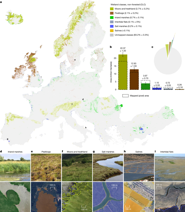
To construct a supervised training dataset from CLC2018, we selected 101,000 training sample points. Each training location was required to be at least 100 m from CLC class boundaries, reducing label noise from neighbouring land-cover types. We defined seven target wetland classes (inland marshes, peatbogs, salt marshes, salines, intertidal flats, moors and heathland and surface water) based on their corresponding CLC classes. For each wetland class c, we drew n_c = 5,000 training sample points, giving a total of

wetland training locations. To represent non-wetland land cover, we drew training sample points from 30 diverse non-wetland and non-water CLC classes, with 2,000 sample points per class, and extra background locations to capture further variability, yielding in total N_background = 66,000 training sample points. The full training set thus comprised N_total = N_wet + N_background = 35,000 + 66,000 = 101,000 training sample points, of which 35,000 represented target wetland classes and 66,000 represented various background (non-wetland and non-water) classes. This stratified design imposed equal sampling effort across wetland classes (5,000 training sample points per class) while also drawing a large and diverse set of background points from many non-wetland land-cover types. At each of the 101,000 training sample locations, we extracted the selected image features (multisensor satellite composites and ancillary layers) using Google Earth Engine¹⁴.

Model selection and optimization

For our wetland type classification task, we selected the XGBoost^13,61 model because of its efficiency and stability for multiclass classification with noisy labels¹³. Let (x_i, y_i) denote training sample i, with feature vector x_i and class label y_i ∈ 1,…, K. XGBoost learns an additive ensemble of regression trees

in which each f_m is a decision tree and M is the number of boosting rounds. At each iteration m, the model is updated as

in which η ∈ (0, 1] is the learning rate. The ensemble is trained by minimizing a regularized objective

in which ℓ(·) is a multiclass loss (softmax) and Ω(f_m) penalizes model complexity (for example, tree depth, number of leaves), which helps control overfitting and improve generalization⁶². Because the coarse CLC labels introduce label noise, some x_iy_i are mislabelled. In gradient boosting, instance weights are implicitly updated by means of the gradient of the loss

so that trees f_m focus on poorly predicted training points while the regularization term Ω(f_m) and learning rate η prevent overfitting to noisy labels. In practice, this means that persistently inconsistent or mislabelled points contribute less to the final decision function, which mitigates the effects of label noise on the CLC-based training set.

We tuned the XGBoost hyperparameters using random search⁶³ with fivefold cross-validation on the training data. For each candidate hyperparameter vector θ_j, we computed a cross-validated loss,

with K = 5 folds and negative mean squared error as the optimization criterion, and retained the configuration with the lowest \(\hat\mathcalL(\boldsymbol\theta _j)\) across 25 candidates (125 fits in total). Cross-validation averages over different training–validation splits, reducing sensitivity to both sampling variability and label noise in the validation folds. The final model used GPU-accelerated boosting with tuned values for the learning rate η = 0.03, maximum tree depth = 9, number of trees M = 1,207, minimum loss reduction (γ) and tree growth policy (depthwise).

After predicting wetland classes at 10-m resolution, we applied a 3 × 3 median (mode) filter to the class map to remove isolated speckle and smooth class boundaries, replacing each pixel label by the most frequent class within its 3 × 3 neighbourhood⁶⁴.

Validation data

We constructed a validation set drawn independently of the training data and not used in model fitting using stratified random sampling with disproportionate allocation, with a minimum of n_c = 500 validation sample points for each target wetland class and a planned total of N_val ≈ 15,000 validation locations across all strata (Supplementary Table 6). All non-target strata (non-wetland and non-water CLC classes) were merged into a single background stratum. Stratum areas were derived by intersecting CLC2018 polygons with the 10-m European Forest Type 2018 dataset⁶⁵, excluding forested regions from the target classes. Within each stratum, we then generated validation sample locations at least 10 m away from all training sample points to ensure spatial independence. Of the planned roughly 15,000 locations, 3,691 could not be placed: the placement algorithm (maximum five attempts per point) could not find positions satisfying the ≥10-m criterion, with the shortfall concentrated in the geometrically narrow salines stratum (208 of 500 planned points generated). A further 326 fell outside the mapped image extent and were removed and eight were excluded during final reference-label quality control because no reliable land-cover label could be assigned, giving N_val = 10,975 sample points.

Each validation sample point was visually interpreted on-screen by an expert using high-resolution Google satellite imagery, following the CLC illustrated nomenclature guidelines⁶⁶, which provide class descriptions, surface-pattern diagrams and example photos to support consistent labelling. Uncertain or ambiguous points were jointly reviewed by two more interpreters until consensus was reached. As contextual information, we consulted the Global Lakes and Wetlands Database v2 (ref. ¹⁵) (for broader wetland system type) and the 10 m Water and Wetness 2018 dataset⁶⁷ (for local patterns of permanent and temporary water and wetness; Supplementary Fig. 9). These ancillary datasets informed interpretation only; final reference labels were assigned solely by expert visual assessment. The sample point retained its original sampling stratum and associated inclusion probability.

Europe-wide area and accuracy estimation

At the European scale, wetland area and map accuracy were estimated directly from the independent continental validation sample N_val = 10,975 using design-based stratified estimation. Area estimation followed a stratified estimator using sampling strata defined by collapsed CLC classes (Supplementary Table 6), consistent with standard practice when reporting classes differ from sampling strata⁶⁸. Let h = 1,…, H index strata with total area A_h and sample size n_h. For reference class k, the within-stratum proportion is

in which I(·) is an indicator function and y_i the reference label. The stratified estimator of class area is

Under stratified random sampling with finite population correction, the variance is

in which N_h = A_h/a is the population size in pixels and a = 100 m² is the pixel area. Standard errors were \(\rmSE(\hatA_k)=\sqrt\rmVar(\hatA_k)\) and 95% confidence intervals were \(\hatA_k\pm 1.96\rmSE(\hatA_k)\). Estimated areas of the population error matrix (Supplementary Tables 7 and 8) were computed analogously for reference class r and mapped class c:

in which m_i is the mapped label and y_i is the reference label. The overall accuracy was

with producer’s and user’s accuracies

To characterize wetland fragmentation from the mapped patch structure, map-defined patch-size bins were derived from contiguous clusters of 10-m cells within each class. The wetland area in each bin was then estimated using the same stratified-design-based indicator estimator as for class-area estimation, with cumulative categories such as <25 ha estimated directly.

Country-level wetland area estimation

Because validation sample sizes for individual wetland classes varied substantially among countries (Supplementary Table 9), direct country-domain estimation alone was often too unstable for reliable reporting and country-level wetland areas were therefore estimated using a calibrated country-level estimator with hierarchical pooling built on the continental stratified probability sample. The domain-estimation motivation follows standard survey-sampling logic for sparse domains⁶⁹, whereas the implemented estimator combines calibration weighting^70,71 with empirical-Bayes compositional pooling^72,73,74. Let h index the continental validation strata and d the reporting countries. To preserve the continental sampling basis, initial expansion weights were defined as

in which A_h is the known total area of stratum h in the analysis frame and n_h is the number of validation sample points in that stratum. To align this continental sample with country-level reporting, these base weights were then calibrated by generalized raking, implemented through iterative proportional fitting, so that the weighted sample matched both the known country frame totals A_d and the known continental stratum totals A_h (refs. ^70,71). In this setting, calibration estimation refers to the adjustment of design-based expansion weights using known auxiliary totals, thereby linking the continental probability sample to the country reporting domains. This calibration step assumes that, after adjusting to known country-frame and stratum-area totals, the calibrated pseudo-counts are conditionally representative of each country’s true class composition. After calibration, weights were normalized within country and normalized weighted class pseudo-counts were computed for each wetland class k as

in which s_d denotes sampled units in country d, \(w_di^\rmnorm\) the normalized calibrated weight and I(·) an indicator for the final reference class. To stabilize country-specific class compositions when these weighted counts were sparse, countries were assigned to fixed macro-regions and region-level mean class compositions were estimated from pooled weighted country counts. We then used a two-level hierarchical empirical-Bayes Dirichlet formulation, in which each country-level class-composition vector π_d was modelled relative to the corresponding macro-regional mean composition μ_r (refs. ^72,73,74). In this hierarchy, country-level compositions are pooled to a shared regional mean for all countries belonging to the same macro-region, with the degree of shrinkage controlled by κ:

in which \(\mathopn\limits^ \sim _d\) is the vector of normalized weighted country reference pseudo-counts, μ_r the corresponding macro-regional mean composition for region r and κ a global shrinkage parameter selected by empirical-Bayes grid search to maximize the Dirichlet-multinomial marginal log-likelihood^72,73,74. This hierarchical formulation preserves positivity and unit-sum constraints and stabilizes weak country estimates by shrinking them towards macro-regional mean compositions, while allowing countries with more informative weighted counts to remain closer to their own observed class composition^72,73. This formulation assumes that countries within each macro-region share broadly similar wetland class compositions (Supplementary Table 9). Posterior draws of π_d were scaled by the known country frame area A_d to obtain country-level class area draws, \(A_d,k^(s)=A_d\pi _d,k^(s)\). Country-level wetland areas were summarized by posterior means and 95% posterior credible intervals.

As a model check, for all 15 countries with effective sample size n_eff ≥ 200 (spanning all five macro-regions), direct calibration-only estimates of total wetland area fell within the 95% posterior credible interval in all cases (mean absolute relative difference 3.2%); for countries with fewer sample points, wider credible intervals reflect appropriately increased uncertainty. For these data-rich countries, low pooling fractions (κ/(κ + n_eff) < 0.12) ensure that country-level calibration data dominate the posterior; the hierarchical structure mainly serves to regularize estimates for countries with sparse validation support, for which direct estimation would be unstable. At the macro-regional level, the aggregate of pooled posterior means across all countries in each of the five regions fell within the 95% posterior credible interval in all cases, with deviations of less than 2.2% from the corresponding direct calibration aggregate.

Wetland disturbance area estimation

Anthropogenic disturbance was defined by intersecting the wetland map with agricultural and urban classes from CLC2018. Wetlands overlapping these classes were classified as most disturbed, those within 150 m of them as intermediately disturbed and all others as least disturbed. Disturbance labels were assigned after sampling and treated as post-stratification reporting domains. Europe-wide areas (EEA38) for disturbance levels and wetland class–disturbance combinations were estimated within the wetland domain using the same stratified indicator estimator described above. At the country level, further post-stratification by disturbance further reduced effective sample sizes within individual wetland classes. Country-level disturbance subdomain areas were therefore estimated by calibrated allocation from the pooled country-level wetland class totals. Let A_c,k denote the pooled country-level area for wetland class k and \(\hatA_k,d^\rmEEA38\) the European design-based area for class k and disturbance level d. The EEA38 disturbance composition within class was defined as

Mapped within-country disturbance shares \(p_c,k,d^\rmmap\) were used as auxiliary information to form initial allocations

These were calibrated within class to satisfy

Calibration was implemented by means of iterative proportional fitting. Uncertainty was propagated by Monte Carlo sampling of pooled country totals and Europe-scale disturbance estimates, with calibration repeated for each draw.

Carbon storage estimation

Sample-based wetland area estimates formed the basis for carbon-stock calculations. At the European scale, stratified class-area estimates derived from the stratified validation sample were used. At the country scale, calibrated hierarchical estimates provided country-level wetland areas. Carbon-density ranges (Mg C ha⁻¹) were compiled from a meta-analysis of 34 studies¹ and harmonized to CORINE wetland classes (Extended Data Table 3). These ranges encompass variability in vegetation, soils, peat depth and land use¹. Although CORINE distinguishes shallow and deep peat, no explicit depth threshold was imposed, as the density ranges used already integrate this variation. For wetland class k, carbon stock (Gt C) was calculated as

in which A_k denotes the sample-based area estimate and \(\rho _k^v\) the minimum, maximum or geometric-mean carbon density. The geometric mean was computed as

motivated by the log-normal behaviour of SOC observed in LUCAS topsoil data (Supplementary Fig. 10). Country-level carbon stocks were obtained by summing across wetland classes.

Adjustment for human disturbances

Disturbance-specific wetland areas were estimated directly. At the European scale, disturbance-domain areas were obtained using the design-based stratified estimator described above. At the country scale, disturbance areas were derived by calibrated allocation from the pooled country-level wetland-class totals, with uncertainty propagated by Monte Carlo sampling of posterior area draws. Carbon densities were adjusted as

in which R_k,d denotes the class-specific reduction factor (Extended Data Table 4). For peatbogs, reductions of 0%, 30% and 50% were assumed for the least, intermediate and most disturbed categories; for other wetland types, reductions of 0%, 20% and 25% were applied. These values were evaluated against LUCAS SOC observations and were conservative relative to observed depletion patterns (Extended Data Fig. 4). Disturbance-adjusted carbon stocks were calculated as

with baseline stocks

Potential carbon stock loss was defined as

and converted to CO₂ equivalents using the molar mass ratio 44/12.

Determining restoration targets

In line with the EU NRL targets under Article 4, we derived scenario-based restoration target areas for (semi)natural open European wetlands failing the ‘good condition’ criteria owing to anthropogenic disturbance using country-level, sample-based disturbance-area estimates. For each country c, disturbed wetland area was defined as the sum of intermediately and most disturbed categories across wetland classes,

and classwise disturbed area as \(\hatA_c,k,\rmdist=\hatA_c,k,1+\hatA_c,k,2\). Restoration targets were then computed as fixed fractions of disturbed area,

with classwise targets defined analogously (\(T_c,k^2030=0.30\,\hatA_c,k,\rmdist\); \(T_c,k^2040=0.60\,\hatA_c,k,\rmdist\)). Given the high carbon density of peatbogs, we also reported peatbog-specific targets based on \(\hatA_c,\rmpeat,\rmdist\). Uncertainty was propagated by applying the same target fractions to each Monte Carlo draw of \(\hatA_c,\rmdist\) and summarizing targets using 95% empirical intervals (Fig. 5 and Supplementary Tables 4 and 5). Finally, we benchmarked the estimated 2030 targets against published national wetland and peatland restoration commitments for the 15 countries with the largest disturbed wetland area, compiled from official policy documents (Extended Data Fig. 5 and Supplementary Table 5).

All analyses were implemented in Python.