Mechanism of age-related accumulation of mtDNA mutations in human blood

Cohorts

UK Biobank

The UKB is a prospective cohort of approximately 500,000 individuals from the UK aged 40–70 years at enrolment, described in more detail elsewhere⁵⁴. The resource includes a vast array of information on each individual, including hospital inpatient diagnoses, questionnaires and surveys collected at the time of enrolment, and several aliquots of peripheral blood. These blood samples are used to obtain estimates of blood cell composition, quantitative levels of blood biomarkers and genomic data. The final tranche of WGS data was recently released, covering virtually everyone in the cohort. This is in addition to whole-exome sequencing (WES) and genotyping array data that also exist for each participant. Pertinent to the present study, the final tranche of WGS data was generated using Illumina NovaSeq 6000 sequencing machines across Sanger and the deCODE facility to an average coverage of 32.5×⁵⁵. All WGS and WES data were accessed using the UKB Research Analysis Platform (RAP) under application 31063.

All of Us

AoU is a large longitudinal cohort intended to capture the diversity of people living in the USA and includes physical measurements, biospecimen collection and survey data on enrolment, as well as capture of electronic health records⁵⁶. For this study, participant data were accessed from the ‘Genetic determinants of mitochondrial DNA phenotypes (v7)’, ‘Genetic determinants of mitochondrial DNA phenotypes (v7) second 40k’, and ‘Genetic determinants of mitochondrial DNA phenotypes (v7) finish pipeline’ workspaces, all of which use the Controlled Data Repository v.7. This data release incorporated WGS data from 245,394 individuals obtained from peripheral blood and sequenced at Baylor College of Medicine, the Broad Institute and the University of Washington. DNA extraction was performed using one of two kits: Autogen or Chemagen.

mtSwirl v2: an updated mtDNA coverage estimation and variant-calling approach

To infer mtCN and accurately call variation on mtDNA, we used mtSwirl, a pipeline we have previously described in more detail⁴. In brief, mtSwirl is a scalable pipeline intended for deployment on cloud platforms for analysis of hundreds of thousands of whole-genome sequences. The pipeline involves initial extraction of unmapped reads, as well as a set of 385 nuclear regions in the GRCh38 reference genome with high homology to mtDNA obtained previously through BLAST (putative nuclear regions of mitochondrial homology, NUMT)⁴. These reads are used to perform an initial pass of variant calling using Mutect2 and HaplotypeCaller for mtDNA and nucDNA, respectively, with GATK v.4.2.6.0. High-confidence homoplasmic and homozygous variation, respectively, are then used to construct a per-individual consensus sequence to which all extracted reads are realigned. Alignment is repeated to a shifted version of the consensus sequence to avoid artificial coverage depression along the edges of the mtDNA sequence. mtDNA variant calling is then repeated using Mutect2, and a custom pipeline is used to map all variant calls and per-base coverage estimates back to GRCh38 for output. In parallel, Haplogrep⁵⁷ is used to perform haplogroup inference.

mtSwirl is intended to be usable on any platform that supports the WDL pipeline language. Owing to substantial limitations of parallelization on UKB RAP, we previously released mtSwirlMulti, which runs multiple samples on individual larger machines. As part of this study, to boost efficiency in UKB, we implemented parallelization within each machine for the most computationally intensive tasks in mtSwirl (SubsetBam, ProcessBamAndRevert, HaplotypeCaller, AlignToMtRegShiftedAndMetrics and LiftoverVCFAndGetCoverage). In effect, our updated version of mtSwirlMulti now implements two layers of parallelization, distributing sets of samples across machines and then using multicore machines to efficiently process the sets of samples in parallel. We ran this new version of mtSwirlMulti on approximately 2,000 samples from the previous release and found that the results were completely identical to those obtained previously. mtSwirlSingle is unchanged from before. We also developed new submission pipelines to efficiently automate job submissions in the UKB RAP and AoU. More details are available at our GitHub repository (https://github.com/rahulg603/mtSwirl).

When used on platforms with a Google Cloud backend (such as AoU Researcher Workbench), the pipeline accesses only the portions of the WGS file relevant for the analysis. Despite this, if WGS data are stored in cold storage (for instance, Nearline), data access charges can be substantial.

We deployed mtSwirlMulti on UKB RAP, processing all of the approximately 300,000 new samples in around 3 weeks given the limit of 100 concurrent machines. We ran mtSwirlSingle across approximately 150,000 new samples in AoU over about 1 week. Within each biobank, new results were merged with mtDNA callsets generated in our previous effort across approximately 250,000 individuals⁴, producing a final, per-biobank mtDNA callset of approximately 500,000 individuals in UKB and approximately 250,000 individuals in AoU.

Sample-level quality control

After variant calls had been completed, samples were removed if:

1. (1)

   the sample showed evidence of abnormally overlapping homoplasmic mutations;

2. (2)

   the sample showed evidence of contamination, assessed by testing whether the sample met any of the following criteria: (a) mtDNA contamination estimate > 2% according to HaploCheck 0124 run by mtSwirl⁵⁸, (b) nucDNA contamination estimate > 2% (obtained as a freemix percentage from the genomic metrics table in AoU and quality control (QC) metrics table from UKB) or (c) multiple haplogroup-defining variants identified at relatively low heteroplasmy;

3. (3)

   the sample was from UKB and was collected during the 2006 pilot analysis.

Derivation of mtCN

The following formula was used to compute raw mtCN:

Mean mtDNA coverage was computed and emitted from the mtSwirl pipeline and was generated from alignment of reads to the per-individual consensus sequence using picard CollectWgsMetrics. In AoU, we obtained mean nucDNA coverage from the genomic metrics file provided in the Controlled Tier v.7. For UKB, as this information was not provided, we computed mean nucDNA coverage using the following formula as described previously⁴:

mtDNA variant QC

For mtDNA variant calls but not mtCN, before variant QC, we also removed any samples with mtCN < 50, as we have previously shown that mtDNA variant count rises in low mtCN samples. This is indicative of potential increased NUMT contamination⁴.

All variants called by Mutect2 were emitted from mtSwirl along with filters obtained using FilterMutectCalls. During merging and annotation, several steps of variant QC were performed once sample filtration had been completed to ensure that our callset was of high quality. Briefly, the steps were as follows.

1. (1)

   Any genotype with a QC filter produced by FilterMutectCalls was removed.

2. (2)

   If heteroplasmy (HL) < 0.01, it was set to homoplasmic recessive.

3. (3)

   If there was no genotype at a site, it was considered homoplasmic recessive provided coverage at that site was at least 100.

4. (4)

   We then removed variants on the basis of heteroplasmy as follows.

   1. (a)

      For analysis of individual common heteroplasmic mutations, we conservatively removed any variants with heteroplasmy less than 0.05 as done previously⁴;

   2. (b)

      For analysis of mtSNV burden, we adopted a more lenient filter to better capture high-confidence low-heteroplasmy variation. which tends to be enriched for age accumulation (Supplementary Note 1). We identified a coverage depth for each person such that 95% of nuclear genomic sites would be expected to have less coverage under a Poisson model. We then removed SNV heteroplasmies with alternative allele depth less than this threshold.

      1. (i)

         As part of the generation of a variant callset for mtSNV burden, we also removed any variants that (in either UKB or AoU) increased by more than 500% relative to an HL > 0.05 filter and were detected more than 30 times. This resulted in exclusion of five suspicious variants: chrM:11467:A:G, chrM:12684:G,A, chrM:12705:C,T, chrM:13052:A,G and chrM:13095:T,C.

mtCN covariate correction

Covariate correction was performed for mtCN as described previously⁴. Briefly, we obtained all blood cell composition percentages within fields 30000–30300, as well as white blood cell count (field 30,000). We (1) excluded lymphocyte percentage owing to collinearity and (2) excluded nucleated RBC percentage as most individuals had zero values. To address outliers, we removed any blood cell measurements that differed from the mean by more than four standard deviations. We also obtained several technical covariates: assessment centre, median blood draw time, fasting time, assessment date and assessment month. To model the nonlinear relationships between mtCN and draw time as well as mtCN and the seasonal effects of assessment date, we used natural splines with five degrees of freedom and seasonally placed knots (3-month increments). Assessment centre and month were modelled as indicator variables. Fasting times between 1 h and 18 h were modelled as indicators as well, with a fasting time of 0 relabelled as 1 and that greater than 18 relabelled as 18 h. All of these variables were included in a joint model:

where ns corresponds to the natural spline function. mtCN_adj was obtained by taking the residuals from the above model. To visualize this residual quantity, we rescaled this value by adding the preadjustment mean of log[mtCN_raw] and then exponentiated to return to absolute scale. As aforementioned, samples obtained during the pilot study in 2006 were excluded.

Construction of mtDNA variant classes

To visualize mtDNA variation as a function of strand, location and mutation type, we considered variants that were between positions 16,172 and 210 to be in the ‘Ori’ region, with all other variants in the ‘Other’ region. As the reference mtDNA genome was the light strand, we considered any variant with a reference allele of C or A to be a light strand variant. For variants with a reference allele of G or T, we took the complement and considered the complement allele to be a heavy strand variant. We considered ‘age-accumulating’ variant classes to comprise those variants that were in the ‘other’ region and were either A>G on either strand or C>T on the heavy strand.

Assessment of mean mtDNA mutation count per person

We performed several analyses in which we considered the mean mtSNV count per person within subcategories of variants (for instance, variant classes or heteroplasmy categories). For these analyses, we counted the number of QC-pass SNVs identified (through the allele-depth-based filter) for each person within each subcategory. The total number of individuals included in this analysis was the number of individuals that passed QC for mtDNA variation assessment. For analyses that considered the mean count per person within subcategories of people (for instance, within age strata) we computed means within defined groups of individuals after quantifying SNV count per person as above within variant subcategories.

In cases where we compared mean SNV counts across variant classes (for instance, that shown in Fig. 2a), we normalized the estimates of mean SNV count across people by the number of possible variants in that variant class to account for differences in the base abundance across mtDNA strand or region. For instance, when comparing the mean variant count per person in the C>T other region on the light versus the heavy strand, we divided the mean observed count in the C>T other region light strand by the total number of possible C>T variants in the other region on the light strand and performed the analogous process for the C>T other region heavy strand.

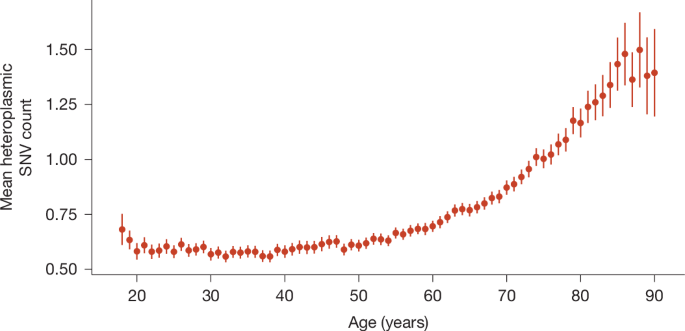
For all analyses in which relationships with age were assessed, only individuals ages 18–90 years (AoU) or 40–70 years (UKB) were included to ensure sufficient samples were retained in age strata.

Analysis of single-base substitution signatures with trinucleotide context

For each variant, trinucleotide context was obtained using the bases immediately 5′ and 3′ to the variant of interest in a strand-specific way. To perform correlations with nucDNA-based single-base substitution signatures, we obtained release v.3.4 of the COSMIC human cancer single-base signatures (SBS) collection¹⁹ (https://cancer.sanger.ac.uk/signatures/downloads/). For each SBS signature, a linear model was fitted to predict the observed mutational spectrum using the SBS signature. P values were reported from the test of significance for the beta coefficient from this model and adjusted for multiple comparisons using the Bonferroni method (two-sided P values, 86 total signatures).

mtDNA variant-based phenotype construction

For analysis of individual common heteroplasmies, we identified all variants that showed QC-pass heteroplasmy (0.05 ≤ HL ≤ 0.95) in 500 or more individuals across both biobanks. This resulted in 78 common heteroplasmic variants selected for analysis. These common mtDNA variants were extracted in each of UKB and AoU, and ‘case-only’ phenotypes were constructed for each heteroplasmy by, for each heteroplasmic variant, marking any individual who failed QC or had a HL of 0 as missing and performing analysis only among those with QC-pass heteroplasmy.

For analysis of heteroplasmic SNVs, we extracted all mtSNVs passing QC with HL ≤ 0.95. We computed SNV burden by counting the number of QC-pass heteroplasmic SNVs per person, retaining people without any recorded QC-pass heteroplasmic SNVs as 0. We also computed an SNV burden trait consisting of the count of age-accumulating class variants only; this was the phenotype on which we performed the bulk of our genetic association analyses.

Family-based analysis in UKB

Relatedness information was obtained for UKB from previous work⁵⁹. All analyses involving related samples were performed using SNVs only. When performing transmission analysis, we only included variants that were identified in at least five individuals to ensure exclusion of artefactual variant calls. When evaluating the degree of heteroplasmic SNV sharing between siblings, we considered a variant to be shared if it was found in both siblings at any heteroplasmy. For each heteroplasmy category, we computed the proportion of variants in sibling 1 (chosen arbitrarily) that were also found in sibling 2.

mtDNA variant consequence annotation and dN/dS estimation

Variant consequences for mtDNA mutations were inferred using VEP v.101 as implemented in Hail. For analysis of mtSNVs, we considered variants labelled as ‘synonymous_variant’, ‘stop_retained_variant’, and ‘non_coding_transcript_exon_variant’ as synonymous; ‘stop_lost’, ‘start_lost’, ‘missense_variant’ as non-synonymous, and ‘stop_gained’ as predicted loss of function.

To estimate dN/dS, we used two approaches. We generated a table of all possible mtSNVs (49,704) and used VEP v.101 to assign mutational consequence. Then, for a given region (such as a gene boundary), we estimated dN as the number of observed non-synonymous variants divided by the number of possible non-synonymous variants within the region and dS as the number of observed synonymous variants divided by the number of possible synonymous variants within the region. The ratio of these two quantities was dN/dS. For all such analyses, we restricted variants to the age-accumulating classes (C>T heavy strand and A>G both strands), as this is the mutational process we were investigating; only this subset of mutations was used for both the observed variants and the count of possible variants (that is, the denominator). In cases in which we generated a variant class- and strand-specific estimate of dN/dS, we restricted variants to the class of interest when counting both observed variants and the count of possible variants. This method was also used in the construction of per-gene dN/dS estimates for mutations found in individuals with detected CH versus in randomly sampled matched controls.

To construct a null distribution under a model of neutrality, we performed random sampling inspired by an approach described elsewhere²³. For each gene and heteroplasmy bin, for each individual i and mutation class c, we randomly sampled \({N}_{i}^{c}\) variants from the set of all possible variants in that gene without replacement, where \({N}_{i}^{c}\) was the number of variants observed for that individual of a specific class within the gene/heteroplasmy bin. This generated a ‘callset’ under the null for which dN/dS was estimated as above. This procedure was repeated 1,000 times to generate a null distribution for dN/dS for each gene, variant class and heteroplasmy range.

As independent validation, we also used the dNdScv package²⁴ to estimate dN/dS for age-accumulating variants. The dndscv command was used with default parameters, including trinucleotide and stranded context, for the mtDNA reference genome using sequence code 2. A 192-rate parameter substitution model was used. The command was run for all age-accumulating class mutations within coding regions within each heteroplasmy bin (that is, it was run separately for each heteroplasmy bin), and gene-specific dN/dS estimates were subsequently obtained from the model outputs.

The genes MT-ATP6 and MT-ATP8 share coding DNA sequence from chrM:8527 to chrM:8572. This meant there was a risk of introducing bias into dN/dS estimates, as mutations within this region face selection forces from two different genes and codon reading frames. Thus, for all dN/dS estimation methods, we corrected for sequence sharing between MT-ATP6 and MT-ATP8 by excluding this region from all stages of the analysis.

UKB disease and smoking phenotype curation

To assess the association of mtDNA phenotypes and common diseases in UKB, we used a previously curated set of 28 common disease phenotypes based on ICD-10 codes, categorical traits curated by UKB and phecodes that spanned several different disease domains⁶⁰. To simplify the cancer terms included in this phenotype set, we constructed two new ICD-10-based traits: haematologic cancer, which involved a diagnosis of C81–C96 or D45–D47; and solid tumour, which involved a diagnosis of C00–C75.

To further evaluate the associations between mtSNV burden and cancer-related phenotypes, we extracted all phecodes with the category of ‘neoplasm’ as curated in previous work⁶⁰. We manually excluded traits corresponding to benign conditions (such as lipoma) or otherwise non-specific traits (for instance, malignant neoplasm other). We filtered to only phenotypes that had more than 140 observed cases in UKB. We obtained smoking status from UKB by obtaining the ID 20116.

Correlation of mtCN and SNV count with disease traits

We computed odds ratios for the associations between mtDNA traits (mtCN, SNV burden) and categorical disease traits using logistic regression as implemented in R in UKB. For all mtDNA traits and disease phenotypes we included genetic ancestry assignment, age, age × sex, age² and age² × sex as covariates, as well as haplogroups as indicator variables. Genetic ancestry groups with fewer than three individuals with any given defined mtDNA trait or disease phenotype were excluded. For analyses in which the independent variable was mtDNA heteroplasmic SNV burden, only age-accumulating variants were used in the burden metric. Individuals who were described as ever having smoked were excluded for all analyses with mtSNV burden.

Correlation of mtCN and SNV count with protein levels and telomere length

We assessed the correlations of mtCN and mtSNV burden with levels of several proteins (FGF21, GDF15, IL1A, IL6, TNF) and telomere length. Proteomics data were obtained as generated and processed by the UKB Pharma Proteomics Project team⁶¹. In brief, UKB plasma samples were obtained and processed through Olink Explore 3072, which provides a platform capable of targeting 2,923 unique proteins. Results were normalized to sample- and plate-specific controls and then corrected for batch. More information can be found using resources 4654–4658 in the UKB Showcase. Field 30900 from UKB contains the normalized proteomics data. For this study, proteomics data were obtained from the 50k release, which was a random subsample of the total UKB population. In terms of further postprocessing, missing data were imputed using the miceforest package as described previously⁶². Telomere length data were also obtained from UKB from field 22192 (‘Z-adjusted T/S log’). These measurements were obtained as described previously⁶³. In brief, DNA from virtually the entire UKB cohort was assayed for telomere length at the University of Leicester by using robot-assisted multiplex qPCR to measure the ratio of telomere repeat copy number relative to a single copy gene. Extensive QC was performed, including removal of samples with a high coefficient of variation and abnormal PCR melt curves. Raw telomere-to-single copy gene ratios were adjusted for several technical factors including batch, machine, temperature, time of day and time-to-collection. Samples were then Z-standardized and log-transformed. As suggested in previous literature⁶³, we adjusted telomere length for white blood cell count using a linear model. This adjusted telomere length was subsequently used for analysis.

Associations between processed telomere length and protein phenotypes and mtCN and mtSNV burden were computed similarly to those done for disease traits. Namely, a linear regression model was used to identify the effect size of changes in mtCN or mtSNV count with respect to telomere length and protein levels while correcting for genetic ancestry assignment, age, age × sex, age², age² × sex and haplogroup. For associations with mtSNV count, we restricted analysis to never-smokers.

Variant-based testing and meta-analysis

In UKB, we performed GWAS using a similar approach to that described previously^4,60. In brief, GWAS was run on GRCh37-based imputed array data using SAIGE v.1.3.6⁶⁴ within previously defined genetic ancestry groups⁶⁰. SAIGE was run using a full genetic relatedness matrix (GRM) in the null model step with leave-one-chromosome-out enabled. All phenotypes were inverse-rank normalized before genetic analysis.

In AoU, we performed GWAS on GRCh38-based WGS data using SAIGE v.1.4.3. We performed extensive sample and variant QC before analysis, in an approach similar to that used by the AoU All-by-All initiative (see https://support.researchallofus.org/hc/en-us/articles/27049847988884-Overview-of-the-All-by-All-tables-available-on-the-All-of-Us-Researcher-Workbench for more details). Unimputed genotype data and WES and WGS data were all used in the generation of files to run SAIGE. Across all data modalities, sample and variant QC were performed as follows. For sample QC, genetic ancestry assignment and ancestry outliers for removal were obtained from the All-by-All effort. Samples were also removed if they were flagged by the AoU DRC. For variant QC, variants were removed if they failed ‘adj’ criteria⁵⁹ or if their ancestry-specific call rate was less than 90%. Ancestry-specific principal components were computed after sample QC on unrelated individuals with projection of related individuals on to the computed principal component space.

To generate the sparse GRM in AoU for each ancestry group, we performed linkage disequilibrium pruning using PLINK on post-QC autosomal genotype data. Linkage disequilibrium pruning was performed using a step size of 1, window size of 10,000 kb, and r2 of 0.1. We excluded the HLA locus and the chromosome 8 inversion locus. Linkage-disequilibrium-pruned genotype data were then exported to PLINK format, and sparse GRMs were constructed within each ancestry with 2,000 markers, a minimum allele frequency of 0.01 and a relatedness cutoff of 0.125 using SAIGE.

Next, to generate files relevant for generation of null models in AoU, we subsampled both WGS and WES data. To ensure that we captured the full range of allele frequencies (given that WGS data were only provided for variants that had allele frequency > 0.01 in at least one ancestry group, that is, ACAF WGS), we obtained 50,000 common autosomal variants at random (allele frequency > 0.01) from WGS data and appended randomly sampled rare variants from WES data. Rare variants were sampled within the following categories: minor allele count (MAC) 1, 2, 3, 4, 5, 6–10, 11–20; minor allele frequency (MAF) < 0.001, MAF < 0.01 and MAF > 0.01. Two-thousand variants were extracted from each MAC category and 10,000 variants were obtained from each MAF category. This was done separately for each population. Linkage disequilibrium pruning was then performed on the combined table of subsampled rare and common variants after removal of HLA and the chromosome 8 inversion locus using r2 0.1 and a window size of 10,000 kb. The resulting pruned variants were exported to PLINK format.

Finally, to efficiently run SAIGE tests, we obtained QC-pass WGS data and then exported BGEN files tiled across the genome separately for each population. This greatly increased parallelism. In AoU, as SAIGE was run with a sparse GRM for improved computational efficiency, leave-one-chromosome-out was disabled.

In both biobanks, all GWAS included ‘baseline’ covariates including the ancestry-specific principal components (10 in UKB, 20 in AoU), age, age × sex, age², and age² × sex. Ancestry groups were only included in the analysis if the analysis had a sample size of 50 or greater. For all mtDNA variant-based analyses (that is, heteroplasmy and SNV burden), we included indicator variables for top-level haplogroup assignments obtained from mtSwirl. We removed any individuals belonging to haplogroups that had fewer than 30 people in either biobank; this resulted in removal of individuals from haplogroups L5, P, Q and S. These were not included for analyses of mtCN. In AoU, a further covariate corresponding to the sequencing site was included. GWAS was always run on phenotypes after inverse-rank normal transformation. Covariate offset was disabled.

For mtDNA heteroplasmy GWAS, we ran analyses using both additive and recessive encoding. In the case of the recessive encoding, BGEN files were re-exported in both biobanks after recoding of heterozygous individuals as homozygous reference. No changes were made in inputs to the null model step.

When GWAS were complete, we performed summary statistics QC. This involved removal of any low-confidence variants (defined as MAC < 20 or call rate < 0.9) and dropping of phenotypes with lambda GC < 1.5. We then performed fixed-effects meta-analysis with inverse-variance weighting within each cohort to meta-analyse populations, followed by another round of fixed-effects meta-analysis with inverse-variance weighting across cohorts. As UKB GWAS was performed in GRCh37, we used a previously generated liftover file to transfer UKB variants to GRCh38 for meta-analysis⁴.

Fine-mapping of UKB GWAS

To identify putative causal variants, we conducted statistical fine-mapping of mtDNA traits in UKB as previously described^4,60,65. Briefly, we used FINEMAP-inf and SuSiE-inf, which model infinitesimal effects⁶⁶, with cross-ancestry meta-analysis summary statistics from UKB and a covariate-adjusted in-sample dosage linkage disequilibrium matrix. To reduce computational burden due to the increased number of genome-wide significant loci, we defined fine-mapping regions on the basis of a 1-Mb window (rather than the previously described 3 Mb^4,60,65) around each lead variant and merged overlapping regions. This resulted in 802 genome-wide significant regions for fine-mapping, of which only 5 loci exceeded 3 Mb, with a maximum length of 5.2 Mb. This approach properly handles long-range linkage disequilibrium regions⁶⁷ while keeping fine-mapping region sizes manageable. We excluded the major histocompatibility complex region (chr6: 25–36 Mb) from analysis, owing to its extensive linkage disequilibrium structure. Allowing up to ten causal variants per region, we derived PIPs using each method with a uniform prior probability of causality and computed the minimum PIP across methods. For 95% credible sets, we used those reported by SuSiE-inf.

Identification of loci and assignment of genes

Owing to the multiancestry and multibiobank nature of our cohort, we used a proximity-based approach to identify separate loci. Specifically, for each GWAS, we identified initial SNVs with P < 5 × 10⁻⁵ and then constructed a window of 100 kb up and down from each such variant. We then iterated through variants in order and merged variants with overlapping windows. A locus was defined as a merged set of variants non-overlapping with any other set, and lead nucDNA variants for a given locus were identified by that with the most significant P value. This process was repeated for published GWAS for CH to obtain lead variants.

For gene assignment, where fine-mapped variants were identified with PIP > 0.1, gene assignment was performed by a combination of nearest gene and manual curation in the genomic region proximal to the fine-mapped variant. Genes in which a protein coding change was predicted by the fine-mapped variant were prioritized. If no fine-mapped variants with PIP > 0.1 were detected, a combination of nearest gene and manual curation was used.

One-sided Mendelian randomization between CH and mtSNV burden

Summary statistics from a recent well-powered case-control analysis of aggregate CH were obtained (GWAS catalogue ID GCST90165261)². Location-based lead variant identification was performed as described above. Odds ratios for lead variants were transformed to log-odds scale, and allele direction was set such that all effect sizes were risk-increasing. Effect sizes and standard errors for these variants from heteroplasmic mtSNV count GWAS were then obtained, ensuring that allele direction was concordant. To determine the statistical significance of the correlation between effect sizes, inverse-variance weighted linear regression was used with weights given by \(1/S{E}_{x}^{2}\times 1/S{E}_{y}^{2}\).

Gene-based testing and meta-analysis

We performed gene-based testing in UKB using the OQFE 500k whole-exome data release. Owing to limited sample sizes for non-European ancestry assigned groups, we performed our analyses using the 500k exome data from individuals of European ancestry only. We used SAIGE-GENE+⁶⁴ v.1.4.3 with identical covariates and phenotypes to those used for variant-based GWAS in UKB. To produce null models, we extracted genotyped variants in the following categories: MAC 1, 2, 3, 4, 5, 6–10, 11–20; MAF < 0.001, MAF < 0.01 and MAF > 0.01. Two-thousand variants were extracted from each MAC category, and 10,000 variants were obtained from each MAF category at random. PLINK was used to perform linkage disequilibrium pruning to obtain a linkage-disequilibrium-independent set of variants for variance ratio estimation. Variance ratios were estimated separately by MAC category, given by MAC 1, 2, 3, 4, 5, 6–10, 11–15, 16–20 and 21+. Assignments of variants to genes and consequence annotations were obtained from previous work⁶⁴.

To perform gene-based testing in AoU, we used the same approaches for variant and sample QC as for variant-based testing. The same sparse GRM was used as well. Analyses were performed in all six ancestry groups. To generate the variant annotation group file, we used the variant annotation table provided by AoU (v.7.1). For each gene, the worst consequence across all transcripts was used to assign each variant to either synonymous, missense or predicted loss of function. Variants with ancestry-wide call rate less than 0.9 were excluded.

To generate null models for rare-variant analysis in AoU, the same input genotypes were used as for common variant analysis, namely a subsampled set of variants with AF > 0.01 using ACAF WGS data combined with subsampled variants with MAC 1, 2, 3, 4, 5, 6–10, 11–20; MAF < 0.001, MAF < 0.01, MAF > 0.01. SAIGE was run with the same parameters as for AoU common variant analysis except with the ‘—isCateVarianceRatio’ option enabled, generating variance ratio estimates for MAC 1, 2, 3, 4, 5, 6–10, 11–15, 16–20 and 21+. These were the same categories used for gene-based testing in UKB.

For parallelism in AoU, we generated BGEN files comprising QC-pass WES-based variant calls tiled across the genome for each population. We adjusted the cut points of these tiles to ensure that gene boundaries were not split across multiple files. These files were used to run SAIGE tests. In AoU, as SAIGE was run with a sparse GRM for improved computational efficiency, leave-one-chromosome-out was disabled.

In both biobanks, a total of 15 tests were performed per gene: maximum MAF values of 0.01, 0.001, and 0.0001; missense/LoF/synonymous, missense/LoF, LoF, missense and synonymous annotations; and a Cauchy combination test combining evidence across annotations. SKAT-O⁶⁸ was primarily used for assessment of gene-based associations. To minimize comparisons, we used the Cauchy test to nominate phenotypes for further evaluation and then evaluated associated variant groups only for those phenotypes. Our genome-wide threshold was set using the Bonferroni method with a threshold of 0.05 divided by ~18,000 corresponding to the number of tested genes, and our ‘suggestive’ threshold was a false discovery rate of 0.1 using the Benjamini–Hochberg procedure.

To conduct cross-ancestry and cross-biobank meta-analysis of gene-based tests, we used both inverse-variance weighted meta-analysis and Stouffer’s weighted P value combination method. Inverse-variance weighting was used to combine burden tests to produce effect size estimates. Stouffer’s weighted P value combination method⁶⁹ was used to combine Burden, SKAT, SKAT-O and Cauchy P values. Weights were constructed as \(\sqrt{N}\), where N is the sample size of a given ancestry or biobank. This meta-analysis procedure was first performed in AoU to combine per-ancestry results and then repeated to combine UKB summary statistics with AoU summary statistics.

Identification of individuals with CH in UKB and AoU

Individuals with CH were obtained from both UKB and AoU as described in detail elsewhere⁷⁰. In brief, CH was identified by assessing for putative somatic variants in WGS data within a curated list of known driver genes for CH by identifying fractional variants with Mutect2, followed by extensive QC and removal of suspected germline variants.

Age- and sex-matching in analyses of individuals with CH

CH is known to be strongly associated with age⁷⁰. Given this, in analyses comparing individuals with detected CH with those without detected CH, we performed age- and sex- matching to minimize the risk of confounding by these variables. We obtained ages and sexes of individuals with known CH and then constructed 500 random samples of people without diagnosed CH of the same size as the CH group. Each of these random samples consisted of people with the same sex and age counts as the CH group. We then computed statistics within each of these control groups (for instance, mean variant count per person within a variant class and age group) and then computed the mean across all random subsamples as the point estimate and the standard deviation of the means across subsamples as the standard error.

For the analysis comparing the normalized mean mutation count between CH and age- and sex-matched controls, we also computed a difference statistic within each random sample; this was the difference in the mean mutation count for a mutation in a particular trinucleotide context between the CH sample and then random sample. We then obtained the point estimate and standard error of the difference statistic using the mean and standard deviation of the difference statistic across all 500 samples, respectively. Significance tests were performed with a null hypothesis of difference of 0 and a two-sided alternative of difference not equal to 0, and P values were corrected using the Bonferroni method assuming 192 comparisons (96 trinucleotide contexts × 2 strands).

Reporting summary

Further information on research design is available in the Nature Portfolio Reporting Summary linked to this article.