


Statistics and reproducibility
Supplementary Table 5 lists the number of independent samples, brains or hemispheres that we examined. All samples are biological replicates. Results were consistent across samples. In cases in which lineages were labelled, numbers indicate total samples collected; however, in some cases a given lineage might not be labelled in every brain. Data grouped together in the same row are from the same samples. If a figure panel is not labelled here, the data are present in its legend.
Number of samples and statistics for Extended Data Fig. 9
For Extended Data Fig. 9e, n = 17 control, 11 mutant and 4 non-induced hemispheres (TfAP-2 RNAi versus control P < 0.0001; TfAP-2 RNAi versus not induced P = 0.0004; control versus not induced P = 0.9989). For Extended Data Fig. 9e′, n = 17 control, 11 mutant and 5 non-induced hemispheres (TfAP-2 RNAi versus control, P < 0.0001; TfAP-2 RNAi versus not induced, P < 0.0001; control versus not induced, P = 0.3209. For Extended Data Fig. 9e,e′: significance, one-way ANOVA with Tukey’s multiple comparisons test.
For Extended Data Fig. 9f,f′,k,k′,l,l′,q,q′,r,r′,s,s′,t,t′,x,y,y′, significance two-sided, unpaired t-test.
For Extended Data Fig. 9f, n = 17 control, 13 mutant and 1 non-induced hemispheres (TfAP-2 RNAi versus control P = 0.0016).
For Extended Data Fig. 9f′, n = 19 control, 14 mutant and 1 non-induced hemispheres (TfAP-2 RNAi versus control P < 0.0001).
For Extended Data Fig. 9k, n = 10 control and 10 experimental hemispheres (P = 0.0043).
For Extended Data Fig. 9k′, n = 6 control and 8 experimental hemispheres (P = 0.0444).
For Extended Data Fig. 9l, n = 16 control and 12 experimental hemispheres (P < 0.0001).
For Extended Data Fig. 9l′, n = 10 control and 8 experimental hemispheres (P = 0.0047).
For Extended Data Fig. 9q, n = 14 control and 18 experimental hemispheres (P = 0.7686).
For Extended Data Fig. 9q′, n = 12 control and 10 experimental hemispheres (P < 0.0001).
For Extended Data Fig. 9r, n = 6 control and 6 experimental hemispheres (P < 0.0001).
For Extended Data Fig. 9r′, n = 10 control and 10 experimental hemispheres (P < 0.0001).
For Extended Data Fig. 9s, n = 14 control and 18 experimental hemispheres (P = 0.0034).
For Extended Data Fig. 9s′, n = 14 control and 19 experimental hemispheres (P < 0.0001).
For Extended Data Fig. 9t,t′, n = 6 control and 6 experimental hemispheres (t, P = 0.7134; t′, P < 0.0001).
For Extended Data Fig. 9x, n = 18 control and 12 experimental hemispheres (P = 0.8401).
For Extended Data Fig. 9y, n = 25 control and 22 experimental hemispheres (P = 0.0002).
For Extended Data Fig. 9y′, n = 25 control and 23 experimental hemispheres (P < 0.0001).
Fly husbandry
Flies were maintained on Bloomington food with a yeast sprinkle (B recipe; Lab Express, Ann Arbor, MI) at 25 °C on a 12:12 light–dark cycle with at least 60% humidity (provided by a beaker of water in the incubator). For staging developmental time points, pupae were marked at the 0 h APF white pre-pupae stage. Animals for scRNA-seq were collected ±1–2 h from the stated developmental time points (for example, 48 h APF were collected from 47–49 h APF). Supplementary Tables 6 and 7 list all genotypes and alleles used in the study and associated references.
Reagents and software
Reagents and software used in this study (as detailed in the sections below) and their associated references are listed in Supplementary Tables 8–14.
Flow cytometry
Flow cytometry to sort GFP-positive neurons from pupal brains was performed similarly to approaches for adult brains45: we pretreated plasticware including tips and Eppendorf tubes with PBS +1% BSA to prevent cells from sticking to the plastic. Dissections of fly brains were performed in Schneider’s +1% BSA for up to 1 h. Optic lobes were removed for the 48 h APF time points. After dissections, collagenase was added to the brains at a concentration of 2 mg ml–1 in Schneider’s 1% BSA, and then placed at 37 °C for 12 min (versus 20 min for adult brains). We then performed a manual dissociation by pipetting the brains up and down at least 30 times, and then spun down the cells at 300 g for 5 min. We removed the supernatant and then resuspended the pellet in 200 μl of PBS +0.1% BSA; we then passed it through a cell strainer cap and spun it down briefly to collect cell suspension at the bottom of the tube. We added 50 ng ml–1 of 4′,6-diamidino-2-phenylindole (DAPI) to our sample and then sorted them into a PBS +1% BSA cushion by using a FACSAria III (University of Michigan BRCF Flow Cytometry Core). During flow cytometry, dead and dying cells were excluded using DAPI signal, and forward and side scatter measurements were used to gate single cells. Scatter profiles consistent with somata (rather than neurite fragments) were determined by back-gating on DAPI. Using our dissociation methods, about 70–90% of singlets seemed viable (DAPI-low) for both time points. As the cells were to be analysed using single-cell sequencing, we set our gates generously (that is, tolerated sorting false positive cells so as to capture all true positives). With these generous gates, about 20% of these viable cells were gated as GFP+ for our 48 h APF time points, and around 2% for 12 h APF. During sorting, we made two adjustments to protect the fly primary cells, which were very delicate: we disabled agitation of the sample tube and sorted using the large nozzle (100 μm; that is, we used larger droplet size and lower pressure).
Single cell RNA sequencing
scRNA-seq library preparation, sequencing and quality control metrics
We prepared eight libraries using the lineage labelling strategy: two replicates at 48 h APF; two replicates at 48 h APF with apoptosis blocked; two replicates at 12 h APF; and two replicates at 12 h APF with apoptosis blocked. At the University of Michigan Advanced Genomics Core, single-cell suspensions collected by flow cytometry were subjected to counting and viability checks on the LUNA Fx7 Automated Cell Counter (Logos Biosystems) and diluted to a concentration of 700–1,000 cells μl–1. Single cell libraries were generated using the 10x Genomics Chromium Controller with 3′ Gene Expression reagents following the manufacturer’s protocol (10x Genomics). As D. melanogaster cells are small, many are lost during the dropletting process; we thus loaded up to 15,000 cells per sample, with the goal of retaining 10,000. Final library quality was assessed using the LabChip GX (PerkinElmer). Libraries were subjected to paired-end sequencing according to the manufacturer’s protocol (Illumina NovaSeq 6000 or Illumina NovaSeqXPlus). We targeted 50,000 reads per cell. Potential doublets and low-quality cells were filtered out by discarding: cells that did not express at least one read for any of our transgenes (lexAop-GFP, lexAop-p35 or LexA-p65), cells with over 50,000 unique molecular identifiers or cells with fewer than 1,000 unique features. The approximately 10% of cells with the highest percentage of mitochondrial transcripts were discarded for all libraries. Features corresponded to genes that were expressed in at least one cell across libraries and were filtered for any mitochondrial genes, transposable elements, ribosomal proteins, mod(mdg4) trans-spliced precursors and non-coding RNAs besides lncRNA:roX1 and lncRNA:roX2 (which are used to assign sex to cells). After filtering, we had a total of 57,076 cells and the number of features used for downstream analyses was 12,957.
scRNA-seq clustering and integration of libraries
We merged all of the libraries and used the Seurat package (Seurat v.5.2.0 or 5.3.0)59 to cluster and integrate our datasets, and to visualize our clusters across conditions (with or without p35) and time points (12 versus 48 h APF). To do this, we normalized gene expression using the ‘NormalizeData’ function (with the ‘LogNormalize’ method). Rather than finding and using the most highly variable genes for the subsequent steps, we used a list of 628 TFs from FlyBase, 609 of which were expressed in our cells. We then scaled our data (ScaleData) while regressing out mitochondrial gene expression (percent.mito) and sequencing depth (nCount_RNA). We then ran principal component analysis using the scaled expression of our 609 TFs (RunPCA) otherwise using default parameters. For clustering and visualizing, we used default parameters, including 50 principal components based on an ElbowPlot (0–200) (‘FindClusters’, ‘FindNeighbors’ and ‘RunUMAP’). We then integrated our datasets (‘IntegrateLayers’) using Harmony Integration and ran the clustering (‘FindClusters’, ‘FindNeighbors’ and ‘RunUMAP’) as we described above to get an idea of the cell types and cell-type diversity that existed in our dataset.
To enrich for non-MB type I hemilineages, we removed Kenyon cells, glia and 12 h APF-specific clusters we found to be optic lobe neurons or progenitor cells (Extended Data Fig. 1). In our top-level clustering, cluster 5 contained Kenyon cells on the basis of the expression of Mef2, ey and dac. Cluster 13 was glia on the basis of the expression of repo. Cluster 3 primarily contained cells from a single library (low-quality cells) and thus we removed it. Seven clusters (20, 15, 6, 22, 46, 27, 43) were specific to the 12 h APF time point and were enriched for scro, but were depleted of Imp and dati (ref. 60), indicating they are optic lobe neurons; we removed these (at 48 h APF, we removed optic lobes during our dissections; at 12 h APF, the optic lobes have not yet separated from the central brain and are thus present during our sorting). Clusters 21 and 47 expressed dpn or dap, were presumed to be progenitor cells, and were therefore removed. Some of these cell types are truly labelled by our recombination-based strategy (progenitors, glia deriving from type I lineages, sporadic clone induction in Kenyon cell lineages). Others are false positives due to a combination of our generous gating and their prevalence. After filtering, we retained a total of 42,844 neurons (18,854 cells from 48 h APF and 23,990 cells from 12 h APF). Extended Data Fig. 1 has the breakdown of how many cells come from each library. To generate the final clustering map we used for biological analyses, we re-ran the workflow above, except that after integrating the datasets, we used a resolution of 1.4 in ‘FindClusters’ determined using ClusTree61. This produced relative stabilization of 56 clusters that we assign as postmitotic neurons originating from cerebral lineages. These are almost all type I lineages; however, we did observe rare labelling of type II sublineages (Supplementary Table 1).
As we describe in the main text, we hypothesize that these clusters mainly corresponded to hemilineages, with larger clusters representing hemilineages always labelled by our lineage trace, and smaller clusters representing hemilineages that were labelled more rarely. That said, as we worked back and forth between the transcriptional to histological points of view, we observed that there was no single clustering resolution that perfectly reflected hemilineage relationships: at lower resolution, some clusters contained multiple hemilineages (for example, anterodorsal and lateral olfactory projection neuron hemilineages), whereas at higher resolution, some hemilineages split into more than one cluster along the birth-order axis. We chose a resolution that kept most hemilineages unified and manually split some of our clusters, as shown in (Extended Data Fig. 1k,l). For example, cluster 0 contained the DAT + CREa1A neurons, which express scro, dmrt99B, erm, D, Lim1, hth, SoxN, CG9932, Sox21b and Fer2, along with other cells that strongly shared Fer2, scro, D, Sox21b, hth and Lim1 but lacked DAT and expressed Gad1 and seemed to be destined to apoptose based on expression of grim. This suggested they are a resurrected hemilineage that typically undergoes apoptosis (programmed cell death, or PCD), which we found experimentally was from SMPad2. We split this cluster into CREa1A and SMPad2_PCD. We also manually split cluster 11 and 41, which contained both Alad1B (adPNs) and a small set of ALl1B/lPNs based on the expression of acj6 (Alad1B/adPNs) versus vvl (ALl1B /lPNs). The matching of transcriptional clusters to hemilineages is described in Supplementary Table 1.
Identifying the lineages labelled by R19C05Pdfr and their hemilineage sisterships
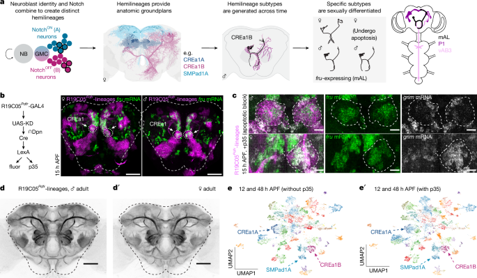
To identify the lineages included in our set of clones, we collected ten male and ten female R19C05Pdfr-lineage trace brains without p35 (natural lineages), and ten male and ten female brains with p35 (which include resurrected cells). We performed IHC against GFP lineage labelling together with neuropil stain with anti-Brp (nc82) to allow image registration. Brains were cleared by mounting in SlowFade Glass. We imaged stained brains at 0.38 μm xy resolution and 1 μm z steps (as for most researchers studying the cerebrum, our z dimension is anterior–posterior) using a 40× oil immersion objective, and registered them to the JRC2018 Unisex common brain template62 using non-rigid registration via CMTK. As GFP in this strategy labels neuronal membranes, we could use both the positions of labelled soma and the morphologies of labelled tracts to identify hemilineages, which we did by comparing to the full adult female brain (FAFB) connectome, for which hemilineages are annotated (see below). For the natural genotype, we took a census of each of the 40 hemispheres (Extended Data Fig. 2c) to determine the labelling rate for each lineage. Overall, we labelled 13 lineages in at least half of brains, and 13 more at least once but fewer than 20 times in our census. This genotype was originally described in a previous work22, in which the authors catalogued ten labelled lineages. We found 8 of these in the set of 26 in our census. We observed a few additional lineages labelled sporadically in our histology experiments that we did not observe among the 26 in our census, and note that our sequencing datasets incorporated about 400 total brains.
Although a number of papers had previously studied cerebral neuron anatomies and origins, adult anatomic hemilineages were systematically named and catalogued in a set of papers published in 2013, and a 2010 census of the lineage origins of fruitless neurons provided additional clonal data for the cerebrum3,8,9,10,63. Two nomenclatures (Ito/Lee versus Hartenstein) were reconciled and anatomic hemilineages were annotated in the FAFB connectome by V. Hartenstein and A. Bates (A. Bates, personal communication)15,64. These annotations have been used to seed hemilineage matches in other connectomes65,66. Most of the annotations in the connectome set include only the secondary parts of hemilineages (that is, the large sets of cells born in the larva); primary neurons, born in the embryo, are mainly categorized as putative_primary, and await association with the rest of their hemilineages. As many have noted, primary neurons share aspects of their anatomy with the secondary parts of their hemilineages, but often have more unique and elaborate innervation patterns, and larger somata67. Morphological subgroups from type II neuroblasts are also typically referred to as sublineages rather than hemilineages, because: (1) there are more than two major morphologies produced by type II lineages; and (2) the lineage tree is structured differently for type II lineages, involving two temporal axes (neuroblast and intermediate progenitor)68,69; however, in the connectome metadata, type II sublineage anatomies are simply called hemilineages (for neuroblasts such as ALl1 that produce more than one major morphology within a hemilineage, those different morphologies may also be referred to as sublineages).
As the two hemilineages from a single neuroblast are generated in parallel (that is, each GMC division produces one neuron for each hemilineage), and because our lineage labelling here is restricted to initiation in Dpn+ cells, there is no way to label one type I hemilineage without labelling its sister (Dpn is also expressed in intermediate progenitors from type II neuroblasts; whereas we find that R19C05Pdfr is mostly restricted to type I neuroblasts, we occasionally label a type II sublineage, as detailed in Supplementary Table 1). Although hemilineages are clonally related and generated in parallel, the two sets of soma are usually pulled apart from one another as their primary neurites grow out along different tracts (this is why the cells expressing hemilineage-specific TFs, like Fer1 in Fig. 2c, are not mingled with their TF-negative sisters); in a minority of cases, the two hemilineages radically separate during metamorphosis (this is why there is sometimes ambiguity in identifying sister hemilineages)8,9,10,63. A survey of 18 type I neuroblasts suggested that around 40% of cerebral type I neuroblasts produce two living hemilineages, whereas 60% produce a lone living hemilineage whose sister hemilineage apoptoses18. The lineage-tracing datasets from 2013 identified many cerebral hemilineage pairs that derive from the same neuroblast. They also provided clues for cases in which a sister is suspected but has not yet been identified, including lineages that produce more than one cell body fibre8, which always occur together9,63, or that produce two first-born neurons observed in the adult10.
Using these clues together with our own clone set, we exhaustively examined whether specific lone hemilineages always occurred together, and are therefore likely to be unidentified sister sets. CLP1 and SLPpm2 were a pair that we newly identified as sisters. We also found cases in which a full living hemilineage is paired with a small set of very different neurons, probably primary neurons of the sister hemilineage (born in the embryo) for which the secondary part of the hemilineage (that is, the large group of neurons born in the larva) apoptosed. PSa1 and SMPad2 are examples of this type of lineage. To find these ‘full hemilineage plus primary neurons of the second hemilineage’ cases, we were aided by: (1) the Cachero 2010 dataset3, which used clonal labelling to identify fruitless cell types from different lineages; (2) descriptions of the central complex cell types and their origins; and (3) images of clones from these and other papers. For example, for PSa1, we saw that the lineage clone for aDT5, which is from PSa1, also includes aDT7 neurons3,8. In the PSa1 clone8, these aDT7 neurons are also visible. In the connectome, aDT7 cells are annotated as ‘putative_primary’, and like most such putative_primary neurons, they are not assigned to a hemilineage. Unlike the annotated PSa1 hemilineage, which are predicted to be GABAergic, aDT7 cells are aminergic. In hemispheres in which we label PSa1, we always label aDT7 cells. We can now assign them as sister to PSa1.
We also examined whether any of our hemilineages of interest in FAFB could be mixtures of two different hemilineages from the same lineage—we looked for cases where an annotated hemilineage included cells with different neurotransmitters that follow distinct outgrowth tracts (Alex Bates, personal communication). We took into account the number of cells annotated to each hemilineage across FAFB, BANC, and maleCNS15,65,66. We also used community annotations in Codex to connect well-studied neurons to their hemilineages.
Finally, we compared our census brains with and without p35, to look for cases of resurrected whole or partial hemilineages. Although this seemed initially like it would be straightforward, we were humbled by the complexity of programmed cell death in brain development, which we understand can occur through at least four routes: first, one of the neurons from each GMC can be programmed to die as it is born, at embryonic or larval stages, as observed by Lin et al.6. Second, some neurons that functioned in the larval brain apoptose during metamorphosis70. Third, neurons can be removed by trophic cell death, that is, when they are overproduced relative to their partners71; while we have not yet observed this in the cerebrum (despite tinkering extensively with ratios of pre- and postsynaptic cells in our work in the mushroom body in Elkahlah et al.72, Ahmed et al.73 and Pan et al., unpublished data), we do not think it should be ruled out. Fourth, there is extensive sex-specific apoptosis in pupal stages26. In summary, we were able to find some clear resurrection of whole hemilineages via ectopic tract morphologies (from the ALv1 and SMPpm1 lineages) and were able to identify the lineage origins of two scRNA-seq clusters containing resurrected neurons (those from PSa1 and SMPad2). Cataloguing which cells apoptose from every lineage/hemilineage and the conditions under which they do so will require extensive further analysis and experimentation.
Clues from the literature and our data and reasoning for lineages in our set are provided in Supplementary Table 1. The references we used to identify lineages/hemilineages and relate them to each other are refs. 3,6,8,9,10,15,18,20,30,63,64,65,66,69,74,75,76,77,78,79,80. Overall, in our 26 lineages, we conclude that one-quarter has two full living hemilineages; one-quarter has one living full hemilineage and a remnant of primary cells from the other hemilineage; and one-quarter has one living full hemilineage and one apoptosing full hemilineage; we did not have enough information to determine the last one-quarter. Three of the anatomic sets that we characterized include so many cells that they probably derive from more than one ‘twin’ neuroblast, SMPad1, SMPad2 and VLPl1_or_VLPl5. For the VLP groups, this is almost certainly the case, as we observe 1n and 2n quanta in different hemispheres.
Matching anatomic hemilineages to transcriptional clusters
Once we had determined the ground truth of which lineages are labelled by our genetic strategy, we began the work of matching anatomic hemilineages to transcriptional scRNA-seq clusters, guided by (and at the same time, testing) the hypothesis that we had clustered neurons in our dataset by hemilineage. We used many types of clues: papers in the literature that had studied TF expression in the pupal or adult brain; markers of neurons that are constituents of these hemilineages, especially fruitless neurons, which are often the best studied representatives of their hemilineage; experimentally determined or electron microscopy-predicted neurotransmitters and the principle that most hemilineages share neurotransmitter usage; patterns of apoptosis in the brain and expression of pro-apoptotic genes in transcriptional space; the expected stoichiometry of different lineages in our dataset; expectation that sister hemilineages would have similar stoichiometry; and the large set of histology experiments performed here, examining hemilineage TFs on the background of R19C05Pdfr-lineage tracing (Fig. 2, Extended Data Fig. 6 and Extended Data Fig. 7). We performed these histology experiments on adults, as we are not yet expert enough anatomists to make hemilineage matches during development. This also confirmed that the hemilineage TFs we identified at 12 h and 48 h APF continue to be expressed in similar patterns in adulthood.
The evidence and reasoning for every match are provided in Supplementary Table 1. We note that almost all of the evidence we amassed was in agreement, and we eventually found explanations for most pieces of data that initially seemed to conflict. Ultimately the process was like the children’s logic puzzle in which one is asked to put characters in order around a table, given clues such as, “Sophie is sitting next to someone wearing a hat, Alfred doesn’t eat vegetables, the child with the hat is eating broccoli, one person is eating spaghetti, and there are no dogs sitting at the dinner table.”
The references we used to learn what cell types are included in hemilineages of interest and to make transcription-to-anatomy matches were as follows: fru or dsx cell memberships within lineages, or their molecular markers3,4,10,22,31,80,81,82,83,84. Other cell-type memberships and molecular markers, by lineage: ALad1 (refs. 35,85,86,87,88,89); CLP1&SLPpm2 (ref. 90); CREa1 (refs. 26,32,33); VESa1 (ref. 30); ALv2 (refs. 14,77,91,92); PSa1 (refs. 3,83); LB7 (ref. 93); SLPpl3 (ref. 17); VLPl1_or_VLPl5 (refs. 80,81); SMPad1 (ref. 32); ALlv1 (refs. 93,94); ALv1 (refs. 85,88,95,96); AOTUv2 (ref. 97); ALl1 (refs. 35,74,76,79,86,87,88,89,95,96,98); LHl2 and LHl4 (ref. 99).
Transcriptional analyses
Subclustering and integration of CREa1B cells
Subclustering was performed using the standard Seurat workflow: gene counts were normalized (using the ‘NormalizeData’ function); 2,000 highly variable genes (FindVariableFeatures) were scaled and used for PCA (using the ‘ScaleData’ and ‘RunPCA’ functions); the first 50 principal components were used for clustering (using the ‘FindNeighbors’ and ‘FindClusters’ functions) and UMAP projections (using the ‘RunUMAP’ function). For integration we used the standard integration workflow of Seurat 5 using Anchor-based canonical correlalation analysis integration to identify shared cell types across time (12 h and 48 h APF). It works by correcting the previously identified PCA coordinates and these corrected coordinates are used for clustering (using the ‘FindNeighbors’ and ‘FindClusters’ functions; resolution = 0.8, clusters = 11) and UMAP projections (using the ‘RunUMAP’ function)59. Clusters 3 and 4 lacked fd59A and TfAP-2. Those cells were removed and the workflow above was re-run (955 cells, resolution = 1.2, clusters = 12). Resolutions were determined using ClusTree.
The proportion of mAL types in males versus females was calculated by dividing the number of pdm3– or br-expressing mALs for each sex by the total number of fru neurons for each condition (with or without p35).
To compare wild-type female mAL neurons and mAL neurons that undergo programmed cell death, first, female mAL neurons were subsetted and then neurons with a high apoptosis signature were determined by UCell using grim, rpr and skl (≥0.04). These were compared with mAL neurons with a low apoptosis signature (<0.04) using the Seurat ‘FindMarkers’ function.
Differentially expressed gene analyses
All differentially expressed gene analyses were performed using the ‘FindMarkers’ function with the default parameters. The differentially expressed genes were then filtered for any non-coding RNAs besides lncRNA:roX1 and lncRNA:roX2; mitochondrial genes; transposable elements; ribosomal proteins; and mod(mdg4) trans-spliced precursors. Plots were made using the ggplot2 package. CREa1B, CREa1A, cluster 0 (SMPad2_PCD), ALad1B (adPNs) and ALl1B (lPNs) marker genes were determined by comparing each of those clusters to all of the other clusters in the dataset (Supplementary Table 2). In the case of CREa1B, clusters were first split by time point, and then marker genes were found as described above (Supplementary Table 2).
Categorizing TF expression (using a computational approach and FindAllMarkers)
We used the FindAllMarkers function from Seurat for the differential gene expression analyses59, using the default Wilcoxon rank-sum test on log-normalized feature counts for our 55 clusters (hemilineage annotated clusters). We selected for TFs that had a minimum percentage difference (min.diff.pct) between the two populations of 50% because we were looking for positive marker TFs for our clusters, resulting in 101 TFs. The results of this analysis are included in Supplementary Table 1 (DEGs (TFs_0.5)).
Categorizing TF expression (manual categorization of TF expression)
For manual categorization of TF expression, we used Seurat’s ‘FeaturePlots’ function to display the expression of the 609 FlyBase TFs that were expressed in at least one cell in our integrated dataset; we split our dataset by time point to discern maturation-based changes in TF expression. We blinded ourselves to gene names, and then categorized each expression pattern as ‘lineage’ (expression in one or more, but not all, whole clusters); ‘order’ or ‘order-like’ (expression in subsets of cells within each cluster); or ‘possibly maturation’ (broad expression, varying across time points). Transcription factors that did not fit into these three simple categories were categorized as either ‘consistent’ (anything that was not differentiated across or within clusters, including near absence of expression, scattered positive cells or pan-neuronal expression); ‘lineage-confusing’ or ‘unclassified/confusing’ (usually a combination of the other axes); ‘Clk-related’ for circadian TFs co-expressed in a small Clk-expressing cluster’; ‘Dsx’ for doublesex; ‘Fru’ for fruitless; and, rarely, multiple labels. Overall, we found 112 putative hemilineage TFs, of which 89 had cluster-defining and -specific expressions without varying over other axes. We identified 35 TFs that we hypothesize reflect birth-order. Our manual descriptions of the expression patterns of each TF are provided in Supplementary Table 3. We manually added chinmo to that list of TFs, due to its known roles in temporal patterning and after re-inspection; it has a gradient, rather than binary, expression, as described in the literature100. This resulted in 36 TFs that we refer to as birth-order TFs. We focused our spatial TF analyses on the 89 TFs with simple cluster-defining expression, as described above, and we refer to them as hemilineage TFs. We note one cluster in which other aspects of patterning won out over hemilineage identity: cluster 4, which is enriched for cells expressing Imp, lov, nub, pdm2 and Kr. Most of these are well-studied early neuroblast temporal factors101,102, suggesting that this is a cluster of primary cells of mixed lineage; additional cells expressing Imp and lov joined typical hemilineage clusters. To confirm that cluster 4 was not a hemilineage, we performed RNA FISH for lov on the R19C05Pdfr-lineage trace background and found that within type I cerebral hemilineages, it labels a subset of cells per clone, not large bundles of soma (Extended Data Fig. 8e). Among the 101 computationally identified TF markers, 82 of those TFs were contained in our list of 89 hemilineage TFs. Ten were called ‘lineage-weird’, and the rest were fru, vri (clk-related) or birth-order TFs. The hemilineage codes in Supplementary Table 1 were determined by filtering the differentially expressed genes identified by Seurat (Supplementary Table 2; all DEGs) for our list of manually identified hemilineage transcription factors.
Lineage variability and temporal dynamicity scores
We also computationally assigned each gene in our dataset a lineage variability score and a temporal dynamicity score (Extended Data Fig. 7u). These scores were calculated using code generously shared by S. Jain and implemented similarly44: we converted our cells into pseudobulk RNA-seq datasets on the basis of their cluster identity and time (cluster 1, 12 h APF; cluster 1 48 h APF, and so on) by aggregating the expression of counts according to cluster and time (AggregateExpression)59. The lineage-variability score was calculated by determining the variance in gene expression across lineages within either time point when the gene was expressed, taking the maximum of those two scores, and then normalizing it by the average expression across cell types at the relevant time point. The temporal dynamicity score was calculated by taking the absolute difference between our 12 h and 48 h time points for each of our hemilineages or clusters in which the gene was expressed, and the averaged value across clusters was then normalized by the average of the peak expression. For a gene to be considered expressed it had to have an aggregated expression level of over 0.2. Both scores had their mean centred to 0 and were transformed to the natural logarithm scale for visualization.
Heatmaps
Heatmaps were made using the ComplexHeatmap package in R in Extended Data Fig. 5 (ref. 103). We identified protein domains enriched within the 89 hemilineage TFs and 36 birth-order TFs using DAVID Bioinformatics Functional Annotation Tool and FlyBase104,105,106. The plots in Fig. 3b,b′ were made by subsetting neurons that express (expression level > 0) either br, pdm3 or mamo but not the other two (expression level == 0).
Pairwise Pearson correlation coefficients between the 36 birth-order TFs (Imp, Syp and fru) based on 12 h APF expression data were computed (cor, method = pearson), and values were hierarchically clustered and visualized using ggcorplot in Fig. 3d. For visualization, Imp was manually set as the first value in an attempt to order cells on the basis of their birth order.
We used the UCell package107 to calculate the gene set enrichment scores at the single-cell level of the following genes: (1) VAChT, DAT, VGlut, Gad1; (2) fru; and (3) rpr, skl and grim. We used the scores to assign our pseudobulk clusters a neurotransmitter identity, whether it is sexually dimorphic on the basis of fru expression, and an apoptosis score. The ranking in UCell uses the Mann–Whitney U statistic.
Variance across versus within clusters versus across time
We calculated the variance in expression for each TF across our pseudobulk clusters grouped by either cluster or time. Median cluster variance was calculated by finding the variance in expression for each TF for each cluster and taking the median value for each TF.
Generation of fly alleles
fruMiMIC[mcherry] (fru-mCherry)
The fruMiMIC[mcherry] flies were made via recombinase-mediated cassette exchange (RMCE) performed by Rainbow Transgenic Flies, with the pBS-KS-attB1-2-GT-SA-mcherry-SV40 vector ordered from the Drosophila Genomics Resource Center108. The DNA was prepared with a Qiagen Plasmid Midi Kit and injected into the original fru[MI05459] line109. Transformants were crossed to yw double-balancer flies and were screened for loss of y+ over the third balancer. As the swap-in construct can incorporate in either direction, we screened F1 progeny of animals positive for loss of the original MiMIC allele for fru-mCherry expression using our two-photon microscope (mCherry has a poor two-photon excitation profile, but we captured the edge of its one-photon excitation using illumination of approximately 700 nm).
Fer1-T2A-Gal4
The Fer1-T2A-GAL4 construct was made using CRISPR/Cas9 homology-directed repair as described in a past work110. The donor cassette was designed to have homology arms of about 1 kb flanking the stop codon (5′ PAM silently mutated, 3′ PAM deleted) with the T2A-GAL4 sequence, taken from Addgene no. 125211 (ref. 111), immediately preceding the stop codon. The donor construct was synthesized and cloned into pBluescript II SK(–) by GENEWIZ from Azenta Life Sciences. Two Fer1 gRNA sequences were generated, as listed in the ‘Oligonucleotides’ section (Supplementary Table 9), and each was synthesized as overlapping primers and annealed to generate dsDNA with BbsI overhangs. Each guide (5′ and 3′) was cloned into pU6-BbsI-chiRNA, generating 5′ and 3′ Fer1 gRNA plasmids. These two plasmids, together with the homology-directed repair donor, were cleaned and injected into y,sc,v; nos-Cas9; +/+ (ref. 112) by Rainbow Transgenic Flies. Injected flies were crossed to double balancers and their progeny were screened by PCR genotyping of amputated legs using the primers listed in the ‘Oligonucleotides’ section (Supplementary Table 9).
Histology and microscopy
Brain dissection and two-photon imaging
Brains were dissected in external saline (108 mM NaCl, 5 mM KCl, 2 mM CaCl2, 8.2 mM MgCl2, 4 mM NaHCO3, 1 mM NaH2PO4, 5 mM trehalose, 10 mM sucrose and 5 mM HEPES at pH 7.5, with the osmolarity adjusted to 265 mOsm). For two-photon imaging, brains were then transferred fresh to 35 mm imaging dishes and pinned to sylgard squares with tungsten wire. Ex vivo two-photon imaging was performed on a Bruker Investigator using a 1.0 NA, 20× water-dipping objective. Stacks were collected along the anterior–posterior axis with 1 μm spacing in z and variable resolution in x and y.
Immunostaining and confocal microscopy
For immunostaining, after dissections brains were transferred to paraformaldehyde in PBS. Brains were fixed overnight at 4 °C in 1% PFA in PBS, or for 25 min at room temperature in 4% PFA in PBS. In general, the 4% PFA method preserves cellular structures better, whereas the 1% PFA method allows better antibody penetration. After same-day (4%) or overnight (1%) fixation, brains were washed three times in PBS supplemented with 0.1% Triton-X-100 on a shaker at room temperature; they were then blocked for at least 1 h in PBS, 0.1% Triton and 4% normal goat serum, and then incubated for at least two nights in primary antibody solution, diluted in PBS, 0.1% Triton and 4% normal goat serum. Primary antibodies were washed three times in PBS supplemented with 0.1% Triton-X-100 on a shaker at room temperature; the brains were then incubated in secondary antibodies for at least two nights, diluted in PBS, 0.1% Triton and 4% normal goat serum. DAPI (1 mg ml–1) was included in secondary antibody mixes. Antibody information can be found in Supplementary Table 8.
Brains were mounted in 1× PBS, 90% glycerol supplemented with propyl gallate or SlowFade mounting medium in binder reinforcement stickers sandwiched between two coverslips. Samples were stored at 4 °C in the dark before imaging. The coverslip sandwiches were taped to slides, allowing us to perform confocal imaging on one side of the brain and then flip over the sandwich to allow a clear view of the other side of the brain. Scanning confocal stacks were collected along the anterior–posterior axis on a Leica SP8 with 1 μm spacing in z and an axial pixel size of about 150 nm, using a 40×, 1.3 NA oil immersion objective. The z dimension corresponds to anterior to posterior dimension of the central brain. For Extended Data Fig. 9h,j, brains were stained and imaged as described in a past work113.
IHC with DPX mounting
In some cases, we sought to improve tissue clarity in IHC experiments using distyrene plasticizer xylene (DPX) mounting. To do this, brains were dissected in dissection saline, and then fixed in cold 4% PFA in PBS for 25 min. Following fixation, brains were washed three times with 0.1% PBS containing 0.1% Triton-X-100 (PBST), and then mounted onto a poly-l-lysine-coated coverslip. Blocking, primary antibody incubation and secondary antibody incubation were performed as described above. After secondary antibody incubation, the samples were washed with 0.1% PBST three times, and then post-fixed with 4% PFA for 2 h at room temperature. After post-fixation, PFA was removed, and samples were washed four times with 0.1% PBST. The tissues were then dehydrated through a graded ethanol series (30%, 50%, 75%, 95% and 2 × 100%), with each step lasting 5 min. This was followed by three washes in xylene (5 min each). Finally, samples were mounted onto glass slides using DPX mounting medium. Mounted slides were air-dried for at least two days at room temperature before confocal imaging; they were then stored at room temperature.
Hybridization chain reaction RNA FISH
RNA FISH experiments were performed as described in a past work114, using hybridization chain reaction (HCR) probe-sets, hairpins and reagents (Molecular Instruments)114,115. Brains were dissected in Schneider’s Drosophila medium and fixed in cold 4% paraformaldehyde in PBS for 20 min at room temperature. Brains were rinsed three times at room temperature in PBS supplemented with 1% Triton-X-100. Samples were pre-hybridized in prewarmed probe hybridization buffer (Molecular Instruments) for 10 min at 37 °C and then incubated with HCR probes in probe hybridization buffer overnight at the same temperature. The next day, they were washed with pre-heated probe wash buffer (Molecular Instruments) and then washed twice in 5× sodium chloride sodium citrate supplemented with 0.1% Tween-20 (SSCT). Samples were then pre-amplified in amplification buffer (Molecular Instruments) for 10–30 min at room temperature and then incubated with snap-cooled HCR hairpins (heated to 95 °C for 90 s before being placed in the dark at room temperature for at least 30 min) in the dark overnight at room temperature. Before washing the brains, 300 μl 5× SSCT was added to the samples to make the solution less viscous. The brains were then washed three times at room temperature first in 5× SSCT, then in probe wash buffer (Molecular Instruments) and then again in 5× SSCT. The brains were then rinsed once in nuclease-free PBS to remove any detergent and then were mounted in 1× PBS, 90% glycerol supplemented with propyl gallate and imaged as described above. In some cases, RNA FISH experiments were performed as described in ref. 116.
Combined RNA FISH and immunohistochemistry
RNA FISH and immunohistochemistry experiments were performed as described in a past work117 using Molecular Instruments HCR probe-sets, hairpins and reagents117. The protein detection stage was first, with care to avoid introducing RNases into the solutions. Brains were dissected in external saline (108 mM NaCl, 5 mM KCl, 2 mM CaCl2, 8.2 mM MgCl2, 4 mM NaHCO3, 1 mM NaH2PO4, 5 mM trehalose, 10 mM sucrose, 5 mM HEPES pH7.5 and osmolarity adjusted to 265 mOsm) and fixed in 4% paraformaldehyde in PBS for 25 min at room temperature. Brains were then washed three times with PBS supplemented with 0.1% Triton-X-100 at room temperature, blocked in antibody buffer (Molecular Instruments) at 4 °C for around 4 h, and then incubated overnight at 4 °C in primary antibody solution in antibody buffer (Molecular Instruments). Samples were then washed four times in PBS supplemented with 0.1% Triton-X-100 at room temperature and incubated in secondary antibody solution made in Antibody Buffer (Molecular Instruments). For some experiments we used the Molecular Instruments initiator labelled secondary antibody to amplify GFP signal (donkey anti-rabbit-B4 for use with amplifier B4) and in other cases we used standard secondary antibodies (goat anti-rabbit-488). Samples were incubated at room temperature for 3 h; they were then washed five times in PBS supplemented with 0.1% Triton-X-100 and once in 5 × SSCT, both at room temperature. Samples then were then post-fixed in 4% paraformaldehyde for 10 min at room temperature, washed twice in PBS supplemented with 0.1% Triton-X-100, and then twice in 5 × SSCT. Samples were then pre-hybridized in probe hybridization buffer for 30 min at 37 °C and then put into a probe mixture made in probe hybridization buffer and incubated at 37 °C overnight. Samples were then washed four times in probe wash buffer at 37 °C and then again in 5 × SSCT at room temperature. Samples were then preamplified in Amplification Buffer (Molecular Instruments) for 10–30 min at room temperature and then incubated with snap-cooled HCR hairpins (95 °C for 90 s and then placed in the dark at room temperature for at least 30 min) in the dark overnight at room temperature. The brains were then washed in 5 × SSCT at room temperature for: (1) 2 × 5 min; (2) 2 × 30 min; and (3) 1 × 5 min. The samples were then mounted as described above.
Alternatively, for R19C05Pdfr clonally labelled brains, we found that GFP was visible after RNA FISH even without immunostaining enhancement. Thus for some RNA FISH experiments on this genetic background, we conducted RNA FISH with care to keep the samples dark, and then imaged enduring native GFP fluorescence to visualize clones.
The following antibodies were used: rabbit anti-GFP (Thermo Fisher Scientific, 1:250 or 1:400), chicken anti-GFP (Dawen Cai lab, 1:5000), rat anti-RFP (Chromtek, 1:400), mouse anti-Br (DSHB, 1:100), guinea pig anti-Mamo (Desplan Lab, 1:200), rat anti-Pdm3 (Desplan Lab, 1:800), guinea pig anti-Otp (Walldorf Lab, 1:400), rat anti-fd59A (Skeath Lab, 1:500 or 1:1,000), mouse anti-ChAT (DSHB, 1:200), rabbit anti-GABA (Sigma, 1:500), mouse anti-nc82 (DSHB, 1:30), guinea pig anti-TfAP-2 (Desplan Lab, 1:100), mouse anti-Acj6 (DSHB, 1:50) and guinea pig anti-Fer2 (1:400, Desplan Lab). Catalogue numbers and references are listed in Supplementary Table 8.
Dye filling of mAL neurons
Dye filling of mAL neurons was performed as previously described27,118. Dye filling electrodes were pulled using a Brown–Flaming puller (Sutter Instruments) and were guided to the mAL axonal tract using fru-GFP. Voltage pulses (50 V pulses, 0.5 ms) were used to electroporate dye into the cells.
Image analysis and statistical considerations
The sexes were separated across experimental conditions because mAL neurons are sexually dimorphic. To count cell populations, we used genetically encoded fluorescence or antibody staining as indicated. We counted labelled somata in every third slice in the stack (every third micron along the anterior–posterior axis), with reference to DAPI to distinguish individual cells from one another. Effect of mutations on axons and dendrites were done in a binary fashion due to the overt changes on brain structures induced by our manipulations, which also made it difficult for the researchers performing quantification to be blinded to experimental conditions. However, analysis was performed blind to the goals of the experiment when possible.
Figure drawings
Drawings of male and female mAL neurons and mlSEZt neurons in Figs. 1a, 2d and 5h were inspired by drawings in a past work119; drawings of their cousins were inspired by CREa1 twin-spot clone data in another past work18. The circuit map in Fig. 1a was inspired by a work by Clowney and co-workers27. Images of hemilineages in Figs. 1a and 2j and Extended Data Fig. 6a,b were screenshotted from Codex (https://codex.flywire.ai) or made using Navis from FAFB dataset15,120,121,122. FlyWire’s public release data is made available under license CC BY-NC 4.0.
Reporting summary
Further information on research design is available in the Nature Portfolio Reporting Summary linked to this article.

